2D Element abundance input file
[25]:
import prodimopy.read as pread
import prodimopy.plot as pplot
import numpy as np
import re
pplot.load_style("nb")
INFO: Load prodimopynb mplstyle from package.
What you need
a prodimo model using you references Elemental abundances (e.g. DIANA)
run it so that you have something to compare
the Element abundances from this model are the reference
with the Elements2D.in we can provide correction factors at each grid point for each element. Those factors are always relative to the initial Element abundances from Elements.in
with this script we generate an Elements2D.in
[26]:
# subroutine to produce the Elements2D.in could be in prodimopy once
# I don't know anymore why it needs to be done this way
def write_elem2D(elemnames,elem2D):
  '''
  Produces the file Elements2D.in in the current directory, in a format compatible with ProDiMo.

  Be careful will overwrite and existing one.
  '''
  print("Write output to Elements2D.in")

  nelem=len(elemnames)

  outstr=str(nelem)+"\n"
  for el in elemnames:
    outstr=outstr+el+" "

  f=open("Elements2D.in","w+")
  f.write(outstr)
  f.write("\n")
  for i in range(nelem):
    f.write(re.sub(r'[\[\]]', '', np.array2string(elem2D[:,:,i],separator=" ",max_line_width=10000,threshold=999999999)))
    f.write("\n")
  f.close()
[27]:
# For this existing model we want to adapt the initial Element Abundances
# can also be a model that was run with stop_after_init. But to compare results a model
# run with the normal Elemental bundances (only Elements.in) would be useful and is recommended.
# also if you need information from the model to produce the new 2D Element abundances a full model
# should be used (e.g. temperature)

################################
# ADAPT THE MODEL DIRECTORY HERE
model=pread.read_prodimo("/home/rab/MODELS/TEST_ELEM2D/TTauri")
READ: Reading File:  /home/rab/MODELS/TEST_ELEM2D/TTauri/ProDiMo.out  ...
READ: Reading File:  /home/rab/MODELS/TEST_ELEM2D/TTauri/Species.out  ...
READ: Reading File:  /home/rab/MODELS/TEST_ELEM2D/TTauri/FlineEstimates.out  ...
READ: Reading File:  /home/rab/MODELS/TEST_ELEM2D/TTauri/Elements.out  ...
READ: Reading File:  /home/rab/MODELS/TEST_ELEM2D/TTauri/dust_opac.out  ...
READ: Reading File:  /home/rab/MODELS/TEST_ELEM2D/TTauri/dust_sigmaa.out  ...
READ: Reading File:  /home/rab/MODELS/TEST_ELEM2D/TTauri/StarSpectrum.out  ...
READ: Reading File:  /home/rab/MODELS/TEST_ELEM2D/TTauri/line_flux.out  ...
WARN: Could not open /home/rab/MODELS/TEST_ELEM2D/TTauri/image.out!
READ: Reading File:  /home/rab/MODELS/TEST_ELEM2D/TTauri/Parameter.out  ...
INFO: Reading time:  0.36 s
[28]:
# those are the initial element abundances from the models, just te be sure they are what we want.
print(model.elements)
name   12    X/H
H     12.000 1.000e+00
He    10.984 9.638e-02
C      8.140 1.380e-04
N      7.900 7.943e-05
O      8.480 3.020e-04
Ne     7.950 8.913e-05
Na     3.360 2.291e-09
Mg     4.030 1.072e-08
Si     4.240 1.738e-08
S      5.270 1.862e-07
Ar     6.080 1.202e-06
Fe     3.240 1.738e-09
PAH    3.444 2.778e-09
Manipulate the Element abundances
Mow we create an array with the correction factors for certain elements. The correction factor is relative to the initial abundances from Elements.in (i.e. 1 means no change)
[29]:
# here we only want to change 2 Elements, the names have to be like in Elements.in
elemnames=["C","O"]
elem2D=np.ones(shape=(model.nx,model.nz,2)) # init it with ones ... no change

# now we make the correction factors
# just as an example we reduce O but increase carbon in the region with A_V<1)
mask=model.AV<1

# now we increase C by a factor of 2 an decrease O by a factor 0.8
elem2D[mask,0]=2.0 # 0 for carbon order like in elemnames from above
elem2D[mask,1]=0.8
[30]:
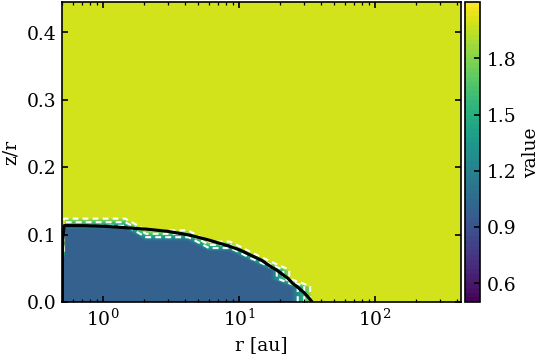
# plot it for checking
pp=pplot.Plot(None)
avcont=pplot.Contour(model.AV,[1],colors="black")
fig=pp.plot_cont(model,elem2D[:,:,0],zlog=False,oconts=[avcont],zlim=[0.5,2.1])
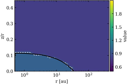
fig=pp.plot_cont(model,elem2D[:,:,1],zlog=False,oconts=[avcont],zlim=[0.5,2.1])
PLOT: plot_cont ...
PLOT: plot_cont ...
[31]:
# now create the File
write_elem2D(elemnames,elem2D)
Write output to Elements2D.in
How to use it
Now copy your initial model to a new model (directory).
copy the generated Elements2D.in into this new model directory
run prodimo for the new model. one can use restart and freeze_RT as the dust RT should not be affacted
quite at the beginning you should see some log statement like this
INIT_ELEMENTS2D: ...
 Use            2 Elements
C   O
this means it detected the file and could read it
compare the result with your initial model
[32]:
# just for checking after running the new model, here called TTauri2ED plot the CO abundance

################################
# ADAPT THE MODEL DIRECTORY HERE
model2D=pread.read_prodimo("/home/rab/MODELS/TEST_ELEM2D/TTauriE2D")
READ: Reading File:  /home/rab/MODELS/TEST_ELEM2D/TTauriE2D/ProDiMo.out  ...
READ: Reading File:  /home/rab/MODELS/TEST_ELEM2D/TTauriE2D/Species.out  ...
READ: Reading File:  /home/rab/MODELS/TEST_ELEM2D/TTauriE2D/FlineEstimates.out  ...
READ: Reading File:  /home/rab/MODELS/TEST_ELEM2D/TTauriE2D/Elements.out  ...
READ: Reading File:  /home/rab/MODELS/TEST_ELEM2D/TTauriE2D/dust_opac.out  ...
READ: Reading File:  /home/rab/MODELS/TEST_ELEM2D/TTauriE2D/dust_sigmaa.out  ...
READ: Reading File:  /home/rab/MODELS/TEST_ELEM2D/TTauriE2D/StarSpectrum.out  ...
READ: Reading File:  /home/rab/MODELS/TEST_ELEM2D/TTauriE2D/line_flux.out  ...
WARN: Could not open /home/rab/MODELS/TEST_ELEM2D/TTauriE2D/image.out!
READ: Reading File:  /home/rab/MODELS/TEST_ELEM2D/TTauriE2D/Parameter.out  ...
INFO: Reading time:  0.36 s
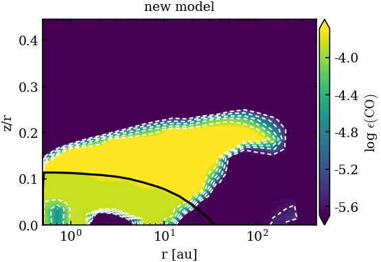
[33]:
avcont=pplot.Contour(model2D.AV,[1],colors="black")
# one should see a difference between the CO abundance above and below the AV=1 line (black)
fig=pp.plot_abuncont(model2D,"CO",zlim=[2.e-6,2.e-4],extend="both",oconts=[avcont],title="new model")
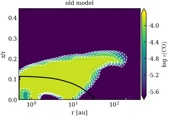
# just the old model as reference
fig=pp.plot_abuncont(model,"CO",zlim=[2.e-6,2.e-4],extend="both",oconts=[avcont],title="old model")
PLOT: plot_abuncont ...
PLOT: plot_abuncont ...