Download this notebook

Plots in one pdf file

This is an example for how to produce on single pdf files with all the figures one wants to plot for a single model. This is similar to the idl script prodimo.pro. prodimopy does not really include something equivalent to prodimo.pro. This here should just show how you can make something similar if you want to.

In that case you can put this code into a python script set the path for read_prodimo to . and call the script within the directory of a prodimo model.

The produced pdf TTauri_new.pdf.

%matplotlib inline
from matplotlib.backends.backend_pdf import PdfPages
import prodimopy.read as pread
import prodimopy.plot as pplot
import os.path

# load a style for notebooks
pplot.load_style("nb")

INFO: Load prodimopynb mplstyle from package.

# Read a model from a directory. Adapt this to your model
model = pread.read_prodimo("~/MODELS/prodimopy/TTauri_new")

# get some information about the model
print(model)

READ: StarSpectrum.out ...
READ: RTinterpolation.out ...
READ: Species.out ...

READ: ProDiMo.out: 100%|██████████| 1600/1600 [00:00<00:00, 16080.57it/s]
READ: FlineEstimates.out: 100%|██████████| 51174/51174 [00:00<00:00, 473284.63it/s]

READ: Elements.out ...
READ: dust_opac.out ...
READ: dust_sigmaa.out ...
READ: line_flux.out ...
READ: SED.out ...
READ: SEDana.out ...
READ: image.out ...
READ: Parameter.out ...
READ: C13O_C12O_ratio.out ...
INFO: Reading time:  0.45 s

Info ProDiMo.out:
NX: 40 NZ: 40 NSPEC: 199 NLAM: 25 NCOOL: 111 NHEAT: 119
p_dust_to_gas: 0.01

Use of PdfPages to create a single pdf with all the figures

# Put a couple of plots to a single pdf
# This puts the output pdf file in the same directory as the model data
# Use `with PdfPages(model.name+".pdf") as pdf:` to put the pdf in the working directory

with PdfPages(os.path.join(".", model.name + ".pdf")) as pdf:
    pp = pplot.Plot(pdf, title=model.name)

    # This plots the Stellar spectrum
    pp.plot_starspec(model, ylim=[1.0e-1, 1.0e11])

    if model.sed is not None:
        pp.plot_sed(model)

    pp.plot_dust_opac(model, ylim=[1.0e-1, None])

    pp.plot_NH(model)

    # you can use latex for the labels!
    # note most of the parameters are optional
    pp.plot_cont(model, model.nHtot, r"$\mathrm{n_{<H>} [cm^{-3}]}$")

    pp.plot_cont(
        model,
        model.nHtot,
        r"$\mathrm{n_{<H>} [cm^{-3}]}$",
        contour=True,
        zr=False,
        xlog=False,
        ylog=False,
        zlim=[1.0e4, None],
        extend="both",
    )
    pp.plot_cont(
        model,
        model.rhod,
        r"$\mathsf{\rho_{dust} [g\;cm^{-3}]}$",
        zr=True,
        xlog=True,
        ylog=False,
        zlim=[1.0e-25, None],
        extend="both",
    )
    pp.plot_cont(
        model,
        model.nd,
        r"$\mathrm{n_{dust} [cm^{-3}]}$",
        contour=True,
        zr=True,
        xlog=True,
        ylog=False,
        zlim=[1.0e-8, None],
        extend="both",
    )

    pp.plot_cont(
        model, model.tg, r"$\mathrm{T_{gas} [K]}$", contour=True, zlim=[5, 5000], extend="both"
    )

    pp.plot_cont(
        model, model.tg, r"$\mathrm{T_{dust} [K]}$", contour=True, zlim=[5, 1500], extend="both"
    )

    # Abundances
    # contour plots for a couple of species
    species = ["CO", "H2O", "HCO+", "HN2+"]
    for spname in species:
        pp.plot_abuncont(
            model, spname, zr=True, xlog=True, ylog=False, zlim=[1.0e-4, 3.0e-15], extend="both"
        )

    # plot the column densityies for those species in a single figure
    pp.plot_cdnmol(model, species)

    # Average abundances
    # plots the average abundances of the above species as a function of radius
    pp.plot_avgabun(model, species, ylim=[3.0e-15, 3.0e-3])

    # Vertical abundances at a certain radius
    # this plots the vertical abundances at different radii for different species
    rs = [10]
    species = ["CO", "HCO+", "e-", "S+"]
    for r in rs:
        pp.plot_abunvert(model, r, species, ylim=[3.0e-15, 3.0e-3])

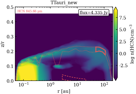
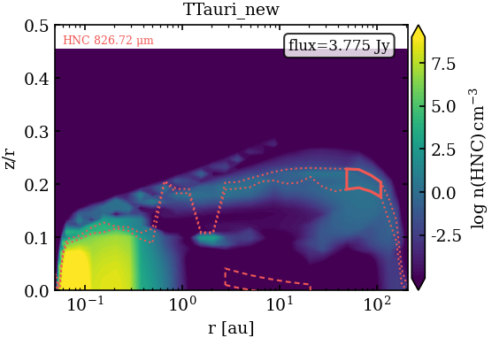
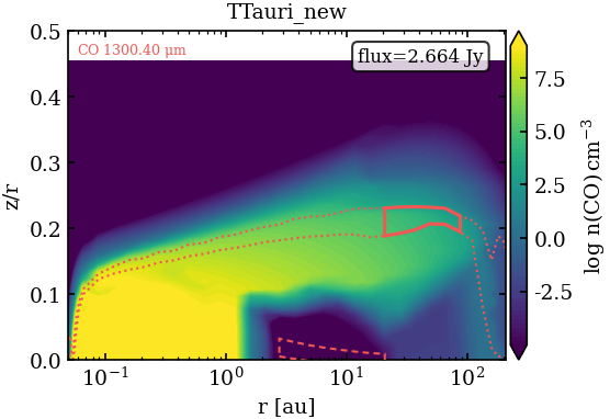
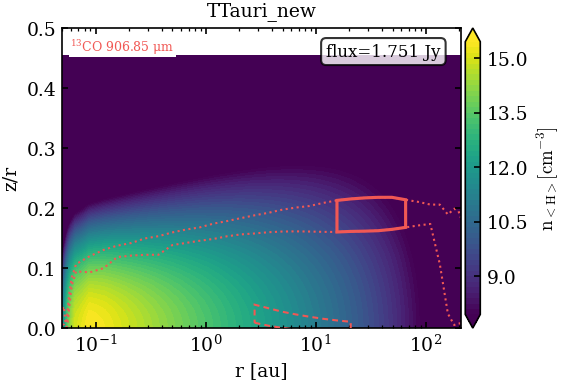
    # get the 10 stronges line fluxes from Fline Estimates at mm wavelengths and plot the line orgins for them
    pptmp = pplot.Plot(None, title=model.name)
    lineests = model.selectLineEstimates(ident=None, wlrange=[800, 1500])
    # sort them
    lineests.sort(key=lambda x: x.flux_Jy, reverse=True)
    nmax = 10
    if len(lineests) < nmax:
        nmax = len(lineests)

    for lineest in lineests[:nmax]:
        # in case the ident really corresponds to a chemical species
        if model.getAbun(lineest.ident) is not None:
            fig = pptmp.plot_line_origin(
                model,
                [[lineest.ident, lineest.wl]],
                model.nmol[:, :, model.spnames[lineest.ident]],
                label=r"log $n(" + pplot.spnToLatex(lineest.ident) + r")\,cm^{-3}$",
                zlim=[1.0e-5, 1.0e9],
                ylim=[None, 0.5],
                extend="both",
                showContOrigin=True,
                showztauD1=False
            )
        else:
            fig = pptmp.plot_line_origin(
                model,
                [[lineest.ident, lineest.wl]],
                model.nHtot,
                label=r"$\mathrm{n_{<H>} [cm^{-3}]}$",
                zlim=[1.0e8, None],
                ylim=[None, 0.5],
                extend="both",
                showContOrigin=True,
                showztauD1=False,
            )

        ax = fig.axes[0]
        props = dict(boxstyle="round", facecolor="white", alpha=0.8)
        ax.text(
            0.95,
            0.95,
            r"flux={:5.3f} Jy".format(lineest.flux_Jy),
            fontsize=8,
            transform=ax.transAxes,
            verticalalignment="top",
            horizontalalignment="right",
            bbox=props,
        )
        pdf.savefig(fig)

    # Line profiles
    # Generate a plot with all the line profiles computed by ProDiMo from LineTransfer.in
    for line in model.lines:
        fig = pp.plot_lineprofile(model, line.wl, loc_legend="upper right")

PLOT: plot_starspec ...
PLOT: plot_sed ...
PLOT: dust opacities ...
PLOT: plot_NH ...
PLOT: plot_cont ...
PLOT: plot_cont ...
PLOT: plot_cont ...
PLOT: plot_cont ...
PLOT: plot_cont ...
PLOT: plot_cont ...
PLOT: plot_abuncont ...
PLOT: plot_abuncont ...
PLOT: plot_abuncont ...
PLOT: plot_abuncont ...
PLOT: plot_cdnmol ...
INFO: Calculate vertical column densities
PLOT: plot_avgabun ...
PLOT: plot_abunvert ...
PLOT: plot_cont ...
PLOT: plot_cont ...
PLOT: plot_cont ...
PLOT: plot_cont ...
PLOT: plot_cont ...
PLOT: plot_cont ...
WARN: getAbun: Species 13CO not found.
PLOT: plot_cont ...
PLOT: plot_cont ...
WARN: getAbun: Species HN13C not found.
PLOT: plot_cont ...
WARN: getAbun: Species HN13C not found.
PLOT: plot_cont ...
PLOT: plot_line_profile ...
PLOT: plot_line_profile ...
PLOT: plot_line_profile ...
PLOT: plot_line_profile ...
PLOT: plot_line_profile ...
PLOT: plot_line_profile ...
PLOT: plot_line_profile ...
PLOT: plot_line_profile ...
PLOT: plot_line_profile ...
PLOT: plot_line_profile ...
PLOT: plot_line_profile ...
PLOT: plot_line_profile ...
PLOT: plot_line_profile ...
PLOT: plot_line_profile ...
PLOT: plot_line_profile ...
PLOT: plot_line_profile ...
PLOT: plot_line_profile ...
PLOT: plot_line_profile ...
PLOT: plot_line_profile ...
PLOT: plot_line_profile ...
PLOT: plot_line_profile ...
PLOT: plot_line_profile ...
PLOT: plot_line_profile ...
PLOT: plot_line_profile ...
PLOT: plot_line_profile ...
PLOT: plot_line_profile ...
PLOT: plot_line_profile ...
PLOT: plot_line_profile ...
PLOT: plot_line_profile ...
PLOT: plot_line_profile ...
PLOT: plot_line_profile ...
PLOT: plot_line_profile ...
PLOT: plot_line_profile ...
PLOT: plot_line_profile ...
PLOT: plot_line_profile ...
PLOT: plot_line_profile ...
PLOT: plot_line_profile ...
PLOT: plot_line_profile ...
PLOT: plot_line_profile ...
PLOT: plot_line_profile ...
PLOT: plot_line_profile ...
PLOT: plot_line_profile ...
PLOT: plot_line_profile ...
PLOT: plot_line_profile ...
PLOT: plot_line_profile ...
PLOT: plot_line_profile ...
PLOT: plot_line_profile ...
PLOT: plot_line_profile ...
PLOT: plot_line_profile ...
PLOT: plot_line_profile ...
PLOT: plot_line_profile ...
PLOT: plot_line_profile ...
PLOT: plot_line_profile ...
PLOT: plot_line_profile ...
PLOT: plot_line_profile ...
PLOT: plot_line_profile ...
PLOT: plot_line_profile ...
PLOT: plot_line_profile ...
PLOT: plot_line_profile ...
PLOT: plot_line_profile ...
PLOT: plot_line_profile ...
PLOT: plot_line_profile ...
PLOT: plot_line_profile ...
PLOT: plot_line_profile ...
PLOT: plot_line_profile ...
PLOT: plot_line_profile ...
PLOT: plot_line_profile ...
PLOT: plot_line_profile ...
PLOT: plot_line_profile ...
PLOT: plot_line_profile ...
PLOT: plot_line_profile ...
PLOT: plot_line_profile ...
PLOT: plot_line_profile ...
PLOT: plot_line_profile ...
PLOT: plot_line_profile ...
PLOT: plot_line_profile ...
PLOT: plot_line_profile ...
PLOT: plot_line_profile ...
PLOT: plot_line_profile ...
PLOT: plot_line_profile ...
PLOT: plot_line_profile ...
PLOT: plot_line_profile ...
PLOT: plot_line_profile ...