0D and 1D Python slab models
Author: Aditya M Arabhavi (arabhavi@astro.rug.nl), adapted by Ch. Rab
Table of contents
0. Importing libraries
Import prodimopy slab library
[1]:
import prodimopy.run_slab as runs # required to run slab models on python, can be skipped if you run
                                  #    models on ProDiMo FORTRAN package
import prodimopy.read_slab as rs # required to read the slab output files
import prodimopy.plot_slab as ps # required to produce plots from the slab data read
import prodimopy.hitran    as ht # useful to digest hitran data if needed for visualization (not required
    #      for reading and plotting prodimo slab models)
import matplotlib.pyplot as plt
import os.path
HAPI version: 1.3.0.0
To get the most up-to-date version please check http://hitran.org/hapi
ATTENTION: Python versions of partition sums from TIPS-2021 are now available in HAPI code

           MIT license: Copyright 2021 HITRAN team, see more at http://hitran.org.

           If you use HAPI in your research or software development,
           please cite it using the following reference:
           R.V. Kochanov, I.E. Gordon, L.S. Rothman, P. Wcislo, C. Hill, J.S. Wilzewski,
           HITRAN Application Programming Interface (HAPI): A comprehensive approach
           to working with spectroscopic data, J. Quant. Spectrosc. Radiat. Transfer 177, 15-30 (2016)
           DOI: 10.1016/j.jqsrt.2016.03.005

           ATTENTION: This is the core version of the HITRAN Application Programming Interface.
                      For more efficient implementation of the absorption coefficient routine,
                      as well as for new profiles, parameters and other functional,
                      please consider using HAPI2 extension library.
                      HAPI2 package is available at http://github.com/hitranonline/hapi2
[2]:
# Setting path to hitran par files
pathHitranPar = "~/git/prodimo/data/HITRAN2020/"
1. Reading the HITRAN data
Data files from HITRAN database can be read using prodimopy.hitran
read_hitran(filePath, moleculeName, isotopologue:list=[1], lowerLam:int=1, higherLam:int=30, sort_label='lambda', quanta=False, format:int=2020, verbose:bool=False)
Older formats of HITRAN can be read by changing the format argument. The default is 2020.
The quantum numbers of the upper and lower global and local levels can also be decoded using quanta=True argument. However, this may fail for some molecules.
The read data is returned in a Pandas DataFrame
[3]:
file = os.path.join(pathHitranPar,"C2H2.par") # Here we use the file from ProDiMo but, the HITRAN files can be downloaded from the HITRAN website.
hit_data = ht.read_hitran(file,moleculeName='C2H2')
hit_data
[3]:
| Molecule_ID | Isotopologue_ID | lambda | nu | S | A | gamma_air | gamma_self | E_u | E_l | ... | del_air | global_u | global_l | local_u | local_l | err_ind | References | line_mixing | g_u | g_l | |
|---|---|---|---|---|---|---|---|---|---|---|---|---|---|---|---|---|---|---|---|---|---|
| 83436 | 26 | 1 | 1.003637 | 9963.76240 | 9.871000e-27 | 0.000546 | 0.0524 | 0.098 | 10918.12720 | 954.3648 | ... | -0.001 | 111 0 2 0 0+ u | 000 0 0 0 0+ g | NaN | R 28e | 356643 | 2219 2 1 1 1 | NaN | 59.0 | 57.0 |
| 83435 | 26 | 1 | 1.003766 | 9962.47770 | 3.929000e-26 | 0.000545 | 0.0541 | 0.101 | 10851.09300 | 888.6153 | ... | -0.001 | 111 0 2 0 0+ u | 000 0 0 0 0+ g | NaN | R 27e | 356643 | 2219 2 1 1 1 | NaN | 171.0 | 165.0 |
| 83434 | 26 | 1 | 1.003901 | 9961.14370 | 1.716000e-26 | 0.000543 | 0.0560 | 0.104 | 10786.34810 | 825.2044 | ... | -0.001 | 111 0 2 0 0+ u | 000 0 0 0 0+ g | NaN | R 26e | 356643 | 2219 2 1 1 1 | NaN | 55.0 | 53.0 |
| 83433 | 26 | 1 | 1.004040 | 9959.76120 | 6.657000e-26 | 0.000542 | 0.0578 | 0.107 | 10723.89420 | 764.1330 | ... | -0.001 | 111 0 2 0 0+ u | 000 0 0 0 0+ g | NaN | R 25e | 356643 | 2219 2 1 1 1 | NaN | 159.0 | 153.0 |
| 83432 | 26 | 1 | 1.004077 | 9959.39620 | 8.536000e-27 | 0.000036 | 0.0733 | 0.132 | 10279.32360 | 319.9274 | ... | -0.001 | 130 0 1 0 1 u | 000 0 0 0 0+ g | NaN | R 16e | 356643 | 2219 2 1 1 1 | NaN | 35.0 | 33.0 |
| ... | ... | ... | ... | ... | ... | ... | ... | ... | ... | ... | ... | ... | ... | ... | ... | ... | ... | ... | ... | ... | ... |
| 5523 | 26 | 1 | 25.165840 | 397.36404 | 3.665000e-28 | 0.000278 | 0.0450 | 0.081 | 3254.21434 | 2856.8503 | ... | -0.001 | 000 2 0 2 0 g | 000 0 1 0 1 u | NaN | P 42f | 345543 | 2320 2 1 1 1 | NaN | 83.0 | 85.0 |
| 5522 | 26 | 1 | 25.325368 | 394.86100 | 6.886000e-28 | 0.000275 | 0.0450 | 0.081 | 3352.75900 | 2957.8980 | ... | -0.001 | 000 2 0 2 0 g | 000 0 1 0 1 u | NaN | P 43f | 345543 | 2320 2 1 1 1 | NaN | 255.0 | 261.0 |
| 5521 | 26 | 1 | 25.460632 | 392.76322 | 1.511000e-28 | 0.000092 | 0.0450 | 0.081 | 3444.88402 | 3052.1208 | ... | -0.001 | 000 2 0 2 0 g | 000 0 1 0 1 u | NaN | P 44e | 345543 | 2320 2 1 1 1 | NaN | 261.0 | 267.0 |
| 5520 | 26 | 1 | 25.487112 | 392.35516 | 1.420000e-28 | 0.000272 | 0.0450 | 0.081 | 3453.62536 | 3061.2702 | ... | -0.001 | 000 2 0 2 0 g | 000 0 1 0 1 u | NaN | P 44f | 345543 | 2320 2 1 1 1 | NaN | 87.0 | 89.0 |
| 5519 | 26 | 1 | 25.651120 | 389.84653 | 2.606000e-28 | 0.000269 | 0.0450 | 0.081 | 3556.81153 | 3166.9650 | ... | -0.001 | 000 2 0 2 0 g | 000 0 1 0 1 u | NaN | P 45f | 345543 | 2320 2 1 1 1 | NaN | 267.0 | 273.0 |
68326 rows × 21 columns
The level format can be retrieved using
getLevelFormat(molecule:str,format:int=2020,level:str='global')
[4]:
ht.getLevelFormat('CO2',
                  format=2020,
                  level='global')
[4]:
'v1 v2 l2 v3 r '
[5]:
ht.getLevelFormat('CO2',
                  format=2020,
                  level='local')
[5]:
'm F '
[6]:
ht.getLevelFormat('CO2',
                  format=2009,
                  level='local')
[6]:
'F '
2. Running 0D models
The run commands/functions for prodimopy are available via prodimopy.run_slab, however are limited to one molecule per model only.
To run the 0D opacity overlap slab models on python the following command can be used
run_0D_slab(Ng, Tg, vturb, molecule, mol_mass, HITRANfile, R_grid, output_filename, isotopolog=[1], wave_mol=[4, 30], wave_spec=[4.9, 28])
Information about what goes into each argument can be found with help(run_0D_slab).
[7]:
help(runs.run_0D_slab)
Help on function run_0D_slab in module prodimopy.run_slab:

run_0D_slab(
    Ng,
    Tg,
    vturb,
    molecule,
    mol_mass,
    HITRANfile,
    cdn_scale_fac=[1],
    custom_partition_sum_file='',
    isotopolog=[1],
    wave_mol=[4, 30],
    wave_spec=[4.9, 28],
    R_grid=100000.0,
    output='both',
    output_filename='default.out',
    mode='both',
    convolve_R=None,
    verbose=True
)
    This is a python implementation of 0D slab models, based on the FORTRAN version of 0D slab models in ProDiMo (https://prodimo.iwf.oeaw.ac.at/)
    This runs models with/without line overlap. More robust and efficient code is available on Fortran, please check the above website (especially for running large grids of models).
    The Fortran code also supports OMP and supports including multiple species.

    Ng : float
        Gas column density (cm-2)

    Tg: float
        Gas temperature (K)

    vturb : float
        Turbulent velocity of the gas (km/s)

    molecule : string or list of strings
        Molecule name, e.g. 'CO2' or ['CO2','C2H2','HCN']

    mol_mass : float or list of floats
        Molecular mass(es) in atomic mass units (amu)

    HITRANfile : string or listt of strings
        Path(s) to the HITRAN '.par' file(s) containing the line data downloaded from HITRAN

    cdn_scale_fac : list of floats
        Column density of the molecules are scaled by these factors (useful for including isotopologue ratios)

    custom_partition_sum_file : string
        Path pointing to file containing custom partition sum (2 columns: temperature, partition sums)

    isotopolog : list
        List containing isotopologue numbers (HITRAN format)

    wave_mol : list
        Wavelength limits in microns to select the lines from the HITRAN file

    wave_spec : list
        Wavelength limits in microns for calculating the spectra

    R_grid : float
        High resolution grid on which the spectra has to be calculated initially
        Recommend minimum of 1e5

    output: string
        'file' to write output to file, 'return' to return a slab type, 'both' for both

    output_filename: string
        Filename(+path) for the output file

    mode : string
        'overlap' or 'line_by_line' or 'both'

    convolve_R : float
        Specrtal resolving power to which the spectra has to be convolved (3500 for JWST/MIRI)

    verbose : boolean
        Whether or not to print progress log
The following demonstrates running a slab model with opacity overlap with parameters:
gas column density = 1e18cm-2,
gas temperature = 250K,
turbulent velocity = 2km/s,
species = CO2,
molecular mass = 44 amu,
HITRAN file of CO2 located at ‘path/to/file.par’,
spectral resolving power = 1e5,
output file = ‘slab_CO2’
This produces a fits output file containing the column of frequency, flux and opacity. The speed on python is low, typically ~3 times slower than on FORTRAN.
[8]:
runs.run_0D_slab(Ng              = 1e18,
                 Tg              = 250,
                 vturb           = 2,
                 molecule        = 'CO2',
                 isotopolog      = [1],
                 mol_mass        = 44,
                 HITRANfile      = os.path.join(pathHitranPar,"CO2.par"),
                 R_grid          = 1e5,
                 wave_mol        = [4,30],
                 wave_spec       = [4.9,28],
                 output          = 'file',
                 output_filename = 'slab_CO2',
                 mode            = 'both',
                 verbose         = True)

# Run a second model with different temperature
runs.run_0D_slab(Ng              = 1e18,
                 Tg              = 500,
                 vturb           = 2,
                 molecule        = 'CO2',
                 isotopolog      = [1],
                 mol_mass        = 44,
                 HITRANfile      = os.path.join(pathHitranPar,"CO2.par"),
                 R_grid          = 1e5,
                 wave_mol        = [4,30],
                 wave_spec       = [4.9,28],
                 output          = 'file',
                 output_filename = 'slab_CO2_T2',
                 mode            = 'both',
                 verbose         = True)
Output written to slab_CO2.fits.gz
Output written to slab_CO2.out
Output written to slab_CO2_T2.fits.gz
Output written to slab_CO2_T2.out
[8]:
()
Line-by-line calculations (i.e., without line overlap) can be performed by setting mode='line_by_line', or only line overlap can be done by setting mode='overlap' or both methods can be done together by mode='both'.
Writing output to a file can be avoided by setting output='return'. This returns a prodimopy.read_slab.slab_data() object containing the calculated model. output='both' writes output to a file as well as returns an object with calculated model.
A user provided partition sums can be used to calculate the lines. The file should be readable by np.loadtxt() containing two columns: temperature and partition sums. The file path should be passed via custom_partition_sum_file argument.
Mutliple molecules can be included in individual slab models. This can be done by including the molecule name, mass, HITRAN file path, column density factor (the column density of the molecule will be scaled by this factor), isotopolog ID. An example is shown below:
[9]:
slab = runs.run_0D_slab(Ng                        = 1e18,
                        Tg                        = 500,
                        vturb                     = 2,
                        molecule                  = ['CO2','CO2'],
                        mol_mass                  = [44,45],
                        HITRANfile                = [os.path.join(pathHitranPar,"CO2.par"),
                                                     os.path.join(pathHitranPar,"CO2.par")],
                        cdn_scale_fac             = [1,1/70],
                        isotopolog                = [1,2],
                        wave_mol                  = [4,30],
                        wave_spec                 = [4.9,28],
                        R_grid                    = 1e5,
                        output                    = 'both',
                        output_filename           = 'slab_CO2_13CO2',
                        mode                      = 'both',
                        convolve_R                = None,
                        verbose                   = True)
Output written to slab_CO2_13CO2.fits.gz
Output written to slab_CO2_13CO2_M0001.out
Output written to slab_CO2_13CO2_M0002.out
The line_by_line output will produce ASCII files for each molecule included. But only one .fits.gz file will be written that accounts for mutual line overlap of all molecules included. If a spectrum of only one species (lets say i, i.e., i=0 for CO2, i=1 for 13CO2 in the above example) but accounting for line overlap is required, this can be done by the .calculate_overlap() method, can be accessed by slabs.models[i].calculate_overlap().
If the molecule is not included in the HITRAN database, or if you intend to use a separate ASCII file containing partition sums, this can be included by passing the file path via the argument custom_partition_sum_file = ‘/path/to/partition/sums/file’. The file should be numpy readable with two columns: temperature and partition sums. When including multiple molecules a list of paths should be passed. For molecules that are in HITRAN, empty string ‘’ can be used in place.
Running a grid of 0D models
A grid of 0D slab models can be run using
run_0D_slab_grid(Ng, Tg, vturb, molecule, mol_mass, HITRANfile, cdn_scale_fac, custom_partition_sum_file, isotopolog, wave_mol, wave_spec, R_grid, output, output_directory, output_filename_prefix, mode, convolve_R, write_index_file, number_of_cores, verbose)
This function follows the same methodology as described in the above text, except the Ng, Tg, vturb are list or numpy.ndarray of equal length and values correspond to each slab model in the grid. Further, the output directory for the files can be specified by output_directory argument. This function appends an index number to the output filenames, the output_filename_prefix is the output filename, but the extensions will be automatically removed if included. write_index_file=True will produce an ASCII file containing the grid point indices and the corresponding Ng, Tg, vturb. To speed up the process, number_of_cores can be specified, which will utilize multiprocessing via specified number of cores. It can take any integer value or “max”, “half”, or “quarter”.
[10]:
import numpy as np
runs.run_0D_slab_grid(Ng                     = np.logspace(17,20,4),
                      Tg                     = np.linspace(300,600,4),
                      vturb                  = np.ones((4))*2,
                      molecule               = ['CO2','CO2'],
                      mol_mass               = [44,45],
                      cdn_scale_fac          = [1,1/70],
                      HITRANfile             = [os.path.join(pathHitranPar,"CO2.par"),
                                                os.path.join(pathHitranPar,"CO2.par")],
                      isotopolog             = [1,2],
                      wave_mol               = [4.9,30],
                      wave_spec              = [4.9,30],
                      R_grid                 = 1e5,
                      output                 = 'return',
                      output_directory       = '.',
                      output_filename_prefix = 'CO2',
                      mode                   = 'overlap',
                      convolve_R             = None,
                      number_of_cores        = 6,
                      verbose                = True)
/home/aditya/anaconda3/envs/jpl/lib/python3.13/multiprocessing/popen_fork.py:67: DeprecationWarning: This process (pid=20623) is multi-threaded, use of fork() may lead to deadlocks in the child.
  self.pid = os.fork()
[10]:
[<prodimopy.read_slab.slab_data at 0xbb93cb60f50>,
 <prodimopy.read_slab.slab_data at 0xbb93cb61090>,
 <prodimopy.read_slab.slab_data at 0xbb93cb60050>,
 <prodimopy.read_slab.slab_data at 0xbb93cb60a50>]
3. Running 1D models
1D models are implemented in ProDiMo FORTRAN package. These models are vertical slab models, see ProDiMo wiki for more information on the code implementation and assumptions.
However, 1D radial models can be run also on python using prodimopy, with the same limitation of only one molecule and no dust opacity. This can be run with:
run_1D_radial_slab(Ng, Tg, R, d, vturb, molecule, mol_mass, HITRANfile, R_grid, output_filename, width='area_given', Rin_limit=0, Rout_limit=1e99, isotopolog=[1], wave_mol=[4,30], wave_spec=[4.9,28])
The description of arguments can be found by help command.
[11]:
help(runs.run_1D_radial_slab)
Help on function run_1D_radial_slab in module prodimopy.run_slab:

run_1D_radial_slab(
    Ng,
    Tg,
    R,
    d,
    vturb,
    R_grid,
    output_filename,
    molecule,
    mol_mass,
    HITRANfile,
    cdn_scale_fac=[1],
    custom_partition_sum_file='',
    width='area_given',
    Rin_limit=0,
    Rout_limit=1e+99,
    isotopolog=[1],
    wave_mol=[4, 30],
    wave_spec=[4.9, 28],
    verbose=False
)
    This is a python implementation of 1D radial slab models, based on the FORTRAN version of 1D slab models in ProDiMo (https://prodimo.iwf.oeaw.ac.at/)
    This runs models with line overlap. More robust and efficient code (including vertical slab model) is available in Fortran, please check the above website (especially for running large grids of models).
    The Fortran code also supports OMP and supports including multiple species.

    Ng : numpy array or list
        Gas column density (cm-2)

    Tg : numpy array or list
        Gas temperature (K)

    R : numpy array or list
        Radius (AU)

    d : float
        Distance of the disk (parsec)

    vturb : float
        Turbulent velocity of the gas (km/s)

    R_grid : float
        High resolution grid on which the spectra has to be calculated initially
        Recommend minimum of 1e5

    output_filename : string
        Filename(+path) for the fits output file
        Use the extension '.fits.gz'

    molecule : string
        Molecule name, e.g. 'CO2'

    molecule : string or list of strings
        Molecule name, e.g. 'CO2' or ['CO2','C2H2','HCN']

    mol_mass : float or list of floats
        Molecular mass(es) in atomic mass units (amu)

    HITRANfile : string or listt of strings
        Path(s) to the HITRAN '.par' file(s) containing the line data downloaded from HITRAN

    cdn_scale_fac : list of floats
        Column density of the molecules are scaled by these factors (useful for including isotopologue ratios)

    custom_partition_sum_file : string
        Path pointing to file containing custom partition sum (2 columns: temperature, partition sums)

    width : string or list or float
        'area_given' - the provided radii array is used as the emitting area equivalent radius
        'infer' - Assumes the provided radius as radial distance from the star and calculates the width of individual rings of slab grids
        list - List containing emitting area equivalent radii
        float - Constant emitting area equivalent radius, used for all grid points

    Rin_limit : float
        Inner radius limit of the disk (AU)

    Rout_limit : float
        Outer radius limit of the disk (AU)

    isotopolog : list
        List containing isotopologue numbers (HITRAN format)

    wave_mol : list
        Wavelength limits in microns to select the lines from the HITRAN file

    wave_spec : list
        Wavelength limits in microns for calculating the spectra
The following shows an example of running a radial slab with 5 grid points.
Note that the computation speed of the model is very low, if large number of models are to be run, e.g. a grid, then running models with the FORTRAN version is highly recommended.
[12]:
runs.run_1D_radial_slab(Ng              = [1e22,1e21,1e20,1e19,1e18],
                        Tg              = [ 650, 450, 350, 300, 250],
                        R               = [0.07, 0.1,0.15, 0.2, 0.5],
                        d               = 190,
                        vturb           = 2,
                        molecule        = 'CO2',
                        mol_mass        = 44,
                        HITRANfile      = os.path.join(pathHitranPar,"CO2.par"),
                        R_grid          = 1e5,
                        output_filename = 'slab_1D_CO2',
                        width           = 'infer',
                        isotopolog      = [1],
                        wave_mol        = [4,30],
                        wave_spec       = [4.9,28])
Same rules apply for including multiple molecules as described in 0D slab model section above
4. Reading and plotting results
The model outputs can be read using the prodimopy.read_slab functions.
[13]:
CO2_0D = rs.read_slab('slab_CO2.fits.gz')
CO2_0DT2 = rs.read_slab('slab_CO2_T2.fits.gz')
CO2_1D = rs.read_slab('slab_1D_CO2.fits.gz')

# convolving the spectra
CO2_0D.convolve(R=3000,lambda_0=4,lambda_n=30,overlap=True)
CO2_0DT2.convolve(R=3000,lambda_0=4,lambda_n=30,overlap=True)
CO2_1D.convolve(R=3000,lambda_0=4,lambda_n=30,overlap=True)
Reading slab line overlap model output from:  slab_CO2.fits.gz
Reading slab line overlap model output from:  slab_CO2_T2.fits.gz
Reading slab line overlap model output from:  slab_1D_CO2.fits.gz

 1 ; Model number  1 ; Species number  None

 1 ; Model number  1 ; Species number  None

 1 ; Model number  1 ; Species number  None
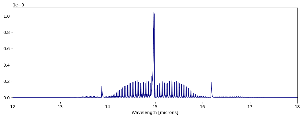
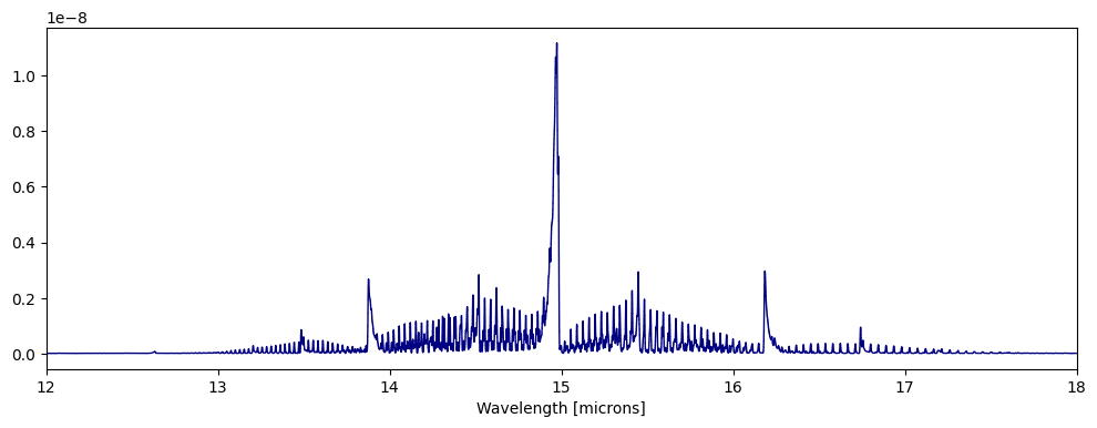
[14]:
fig,ax=plt.subplots(figsize=(12,4))
ps.plot_spectra(CO2_0D,overlap=True,fig=fig,ax=ax)
ax.set_xlim([12,18])

fig,ax=plt.subplots(figsize=(12,4))
ps.plot_spectra(CO2_0DT2,overlap=True,fig=fig,ax=ax)
ax.set_xlim([12,18])
[14]:
(12.0, 18.0)
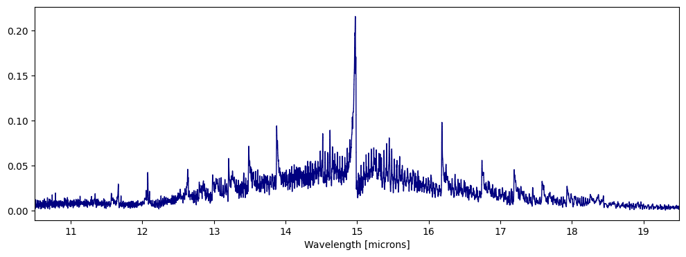
[15]:
jansky = 1e23
fig,ax = plt.subplots(figsize=(12,4))
ps.plot_spectra(CO2_1D,overlap=True,scaling=jansky,fig=fig,ax=ax)
ax.set_xlim([10.5,19.5])
[15]:
(10.5, 19.5)
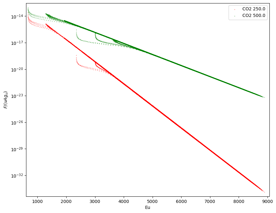
5. Plotting Boltzmann diagram
plotBoltzmannDiagram(data,ax=None,fig=None,figsize=None,NLTE=False,label=None,s=0.1,c='k',set_axis_limits=True)
[16]:
data=rs.read_slab("slab_CO2.out")
dataT2=rs.read_slab("slab_CO2_T2.out")
fig,ax = ps.plotBoltzmannDiagram([data,dataT2],
                                 c=['r','g','b'],
                                 label=[d.species_name+' '+str(d.Tg) for d in [data,dataT2]],
                                 figsize=(10,8))
Reading slab model output from:  slab_CO2.out
Reading slab model output from:  slab_CO2_T2.out
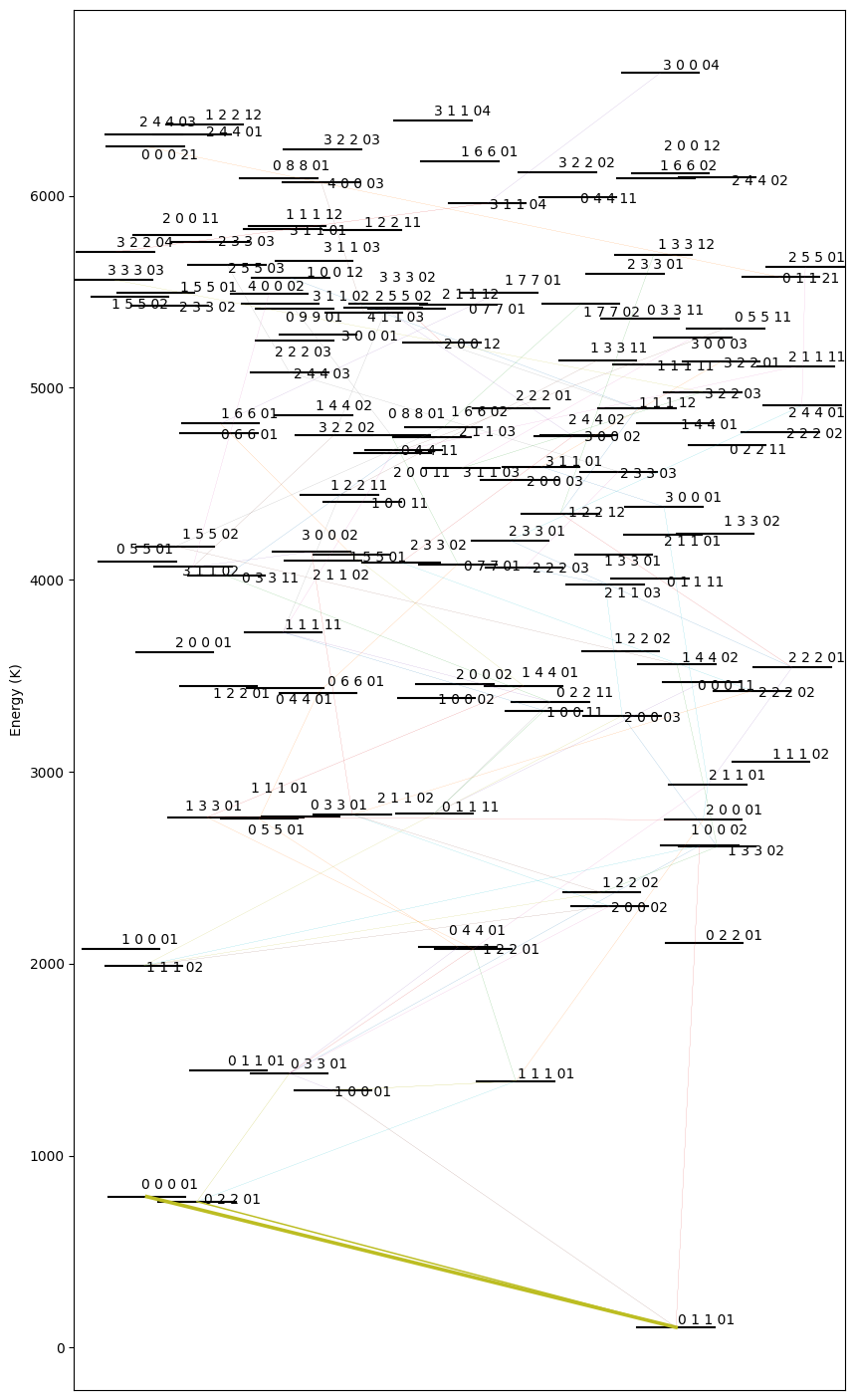
6. Plotting energy level diagram
plotLevelDiagram(data,ax=None,figsize=(10,18),seed=None,lambda_0=None,lambda_n=None,width_nlines=False)
This function takes in only 1 slab model at a time. The arrangement of the levels along the x axis is random, hence the function also returns the seed used to generate it (also prints). The seed can be passed as an argument to retrieve the same arrangement of levels again.
The thickness of the line is proportional to the total flux that band is contributing. width_nlines can be set to True to make the line thickness proportional to the number of lines in that band.
lambda_0 and lambda_n can be used to focus on certain spectral region to make the level diagram. This can be helpful to analyse which bands are contributing to a certain spectral feature.
[17]:
fig,ax,seed = ps.plotLevelDiagram(data,lambda_0=14.5,lambda_n=14.7) # try this seed 7153029
Random seed = 22633712