More complex examples
of using prodimopy slab libraries
Author: Aditya M Arabhavi (arabhavi@astro.rug.nl) Last Updated: July 24, 2023 Read the docs: prodimopy
Table of contents
2. Slicing, indexing and retrieving data from the read models
-
8. 1D Models with ProDiMo and prodimopy
0. Importing libraries and downloading example output
Import prodimopy slab library
[1]:
import prodimopy.run_slab as runs # required to run slab models on python, can be skipped if you run
                                  #    models on ProDiMo FORTRAN package
import prodimopy.read_slab as rs # required to read the slab output files
import prodimopy.plot_slab as ps # required to produce plots from the slab data read
import prodimopy.hitran    as ht # useful to digest hitran data if needed for visualization (not required
    #      for reading and plotting prodimo slab models)
import matplotlib.pyplot as plt
OMP: Warning #182: OMP_STACKSIZE: ignored because GOMP_STACKSIZE has been defined
Download example output (Needs to be done only once) Contains slab model output with three temperatures 200K, 500K, 900K for two molecules C2H2 and HCN
[2]:
%%bash
wget https://raw.githubusercontent.com/adityamarabhavi/prodimopy/main/example/output_files/SlabResults.out
--2025-02-06 12:04:43--  https://raw.githubusercontent.com/adityamarabhavi/prodimopy/main/example/output_files/SlabResults.out
Resolving raw.githubusercontent.com (raw.githubusercontent.com)... 185.199.109.133, 185.199.108.133, 185.199.110.133, ...
Connecting to raw.githubusercontent.com (raw.githubusercontent.com)|185.199.109.133|:443... connected.
HTTP request sent, awaiting response... 200 OK
Length: 14183573 (14M) [text/plain]
Saving to: ‘SlabResults.out.2’

     0K .......... .......... .......... .......... ..........  0% 5.24M 3s
    50K .......... .......... .......... .......... ..........  0% 6.01M 2s
   100K .......... .......... .......... .......... ..........  1% 35.5M 2s
   150K .......... .......... .......... .......... ..........  1% 33.3M 1s
   200K .......... .......... .......... .......... ..........  1% 9.04M 1s
   250K .......... .......... .......... .......... ..........  2% 32.8M 1s
   300K .......... .......... .......... .......... ..........  2% 52.8M 1s
   350K .......... .......... .......... .......... ..........  2% 41.8M 1s
   400K .......... .......... .......... .......... ..........  3% 51.0M 1s
   450K .......... .......... .......... .......... ..........  3% 86.3M 1s
   500K .......... .......... .......... .......... ..........  3% 10.4M 1s
   550K .......... .......... .......... .......... ..........  4% 99.1M 1s
   600K .......... .......... .......... .......... ..........  4% 57.2M 1s
   650K .......... .......... .......... .......... ..........  5%  119M 1s
   700K .......... .......... .......... .......... ..........  5%  141M 1s
   750K .......... .......... .......... .......... ..........  5% 93.6M 1s
   800K .......... .......... .......... .......... ..........  6% 92.0M 1s
   850K .......... .......... .......... .......... ..........  6%  119M 1s
   900K .......... .......... .......... .......... ..........  6% 94.8M 1s
   950K .......... .......... .......... .......... ..........  7%  155M 1s
  1000K .......... .......... .......... .......... ..........  7% 14.8M 1s
  1050K .......... .......... .......... .......... ..........  7%  119M 1s
  1100K .......... .......... .......... .......... ..........  8% 54.2M 0s
  1150K .......... .......... .......... .......... ..........  8% 98.1M 0s
  1200K .......... .......... .......... .......... ..........  9%  131M 0s
  1250K .......... .......... .......... .......... ..........  9%  104M 0s
  1300K .......... .......... .......... .......... ..........  9%  114M 0s
  1350K .......... .......... .......... .......... .......... 10%  136M 0s
  1400K .......... .......... .......... .......... .......... 10%  107M 0s
  1450K .......... .......... .......... .......... .......... 10% 88.0M 0s
  1500K .......... .......... .......... .......... .......... 11%  105M 0s
  1550K .......... .......... .......... .......... .......... 11%  176M 0s
  1600K .......... .......... .......... .......... .......... 11%  115M 0s
  1650K .......... .......... .......... .......... .......... 12%  110M 0s
  1700K .......... .......... .......... .......... .......... 12% 92.3M 0s
  1750K .......... .......... .......... .......... .......... 12%  136M 0s
  1800K .......... .......... .......... .......... .......... 13%  101M 0s
  1850K .......... .......... .......... .......... .......... 13%  123M 0s
  1900K .......... .......... .......... .......... .......... 14%  101M 0s
  1950K .......... .......... .......... .......... .......... 14%  130M 0s
  2000K .......... .......... .......... .......... .......... 14%  115M 0s
  2050K .......... .......... .......... .......... .......... 15% 88.6M 0s
  2100K .......... .......... .......... .......... .......... 15%  121M 0s
  2150K .......... .......... .......... .......... .......... 15%  103M 0s
  2200K .......... .......... .......... .......... .......... 16%  137M 0s
  2250K .......... .......... .......... .......... .......... 16%  108M 0s
  2300K .......... .......... .......... .......... .......... 16% 99.1M 0s
  2350K .......... .......... .......... .......... .......... 17%  146M 0s
  2400K .......... .......... .......... .......... .......... 17%  115M 0s
  2450K .......... .......... .......... .......... .......... 18% 91.5M 0s
  2500K .......... .......... .......... .......... .......... 18%  117M 0s
  2550K .......... .......... .......... .......... .......... 18%  145M 0s
  2600K .......... .......... .......... .......... .......... 19% 97.8M 0s
  2650K .......... .......... .......... .......... .......... 19%  108M 0s
  2700K .......... .......... .......... .......... .......... 19% 99.3M 0s
  2750K .......... .......... .......... .......... .......... 20%  104M 0s
  2800K .......... .......... .......... .......... .......... 20%  154M 0s
  2850K .......... .......... .......... .......... .......... 20%  106M 0s
  2900K .......... .......... .......... .......... .......... 21%  103M 0s
  2950K .......... .......... .......... .......... .......... 21% 1.84M 0s
  3000K .......... .......... .......... .......... .......... 22%  128M 0s
  3050K .......... .......... .......... .......... .......... 22%  135M 0s
  3100K .......... .......... .......... .......... .......... 22%  129M 0s
  3150K .......... .......... .......... .......... .......... 23%  179M 0s
  3200K .......... .......... .......... .......... .......... 23%  237M 0s
  3250K .......... .......... .......... .......... .......... 23%  224M 0s
  3300K .......... .......... .......... .......... .......... 24%  264M 0s
  3350K .......... .......... .......... .......... .......... 24%  250M 0s
  3400K .......... .......... .......... .......... .......... 24%  281M 0s
  3450K .......... .......... .......... .......... .......... 25%  278M 0s
  3500K .......... .......... .......... .......... .......... 25%  234M 0s
  3550K .......... .......... .......... .......... .......... 25%  144M 0s
  3600K .......... .......... .......... .......... .......... 26%  168M 0s
  3650K .......... .......... .......... .......... .......... 26%  223M 0s
  3700K .......... .......... .......... .......... .......... 27%  215M 0s
  3750K .......... .......... .......... .......... .......... 27%  246M 0s
  3800K .......... .......... .......... .......... .......... 27%  281M 0s
  3850K .......... .......... .......... .......... .......... 28%  234M 0s
  3900K .......... .......... .......... .......... .......... 28%  278M 0s
  3950K .......... .......... .......... .......... .......... 28%  217M 0s
  4000K .......... .......... .......... .......... .......... 29%  232M 0s
  4050K .......... .......... .......... .......... .......... 29%  281M 0s
  4100K .......... .......... .......... .......... .......... 29%  201M 0s
  4150K .......... .......... .......... .......... .......... 30%  145M 0s
  4200K .......... .......... .......... .......... .......... 30%  205M 0s
  4250K .......... .......... .......... .......... .......... 31%  274M 0s
  4300K .......... .......... .......... .......... .......... 31%  240M 0s
  4350K .......... .......... .......... .......... .......... 31%  235M 0s
  4400K .......... .......... .......... .......... .......... 32%  251M 0s
  4450K .......... .......... .......... .......... .......... 32%  267M 0s
  4500K .......... .......... .......... .......... .......... 32%  262M 0s
  4550K .......... .......... .......... .......... .......... 33%  249M 0s
  4600K .......... .......... .......... .......... .......... 33%  250M 0s
  4650K .......... .......... .......... .......... .......... 33%  285M 0s
  4700K .......... .......... .......... .......... .......... 34%  283M 0s
  4750K .......... .......... .......... .......... .......... 34%  212M 0s
  4800K .......... .......... .......... .......... .......... 35%  284M 0s
  4850K .......... .......... .......... .......... .......... 35%  248M 0s
  4900K .......... .......... .......... .......... .......... 35%  284M 0s
  4950K .......... .......... .......... .......... .......... 36%  203M 0s
  5000K .......... .......... .......... .......... .......... 36%  272M 0s
  5050K .......... .......... .......... .......... .......... 36%  285M 0s
  5100K .......... .......... .......... .......... .......... 37%  237M 0s
  5150K .......... .......... .......... .......... .......... 37%  160M 0s
  5200K .......... .......... .......... .......... .......... 37%  155M 0s
  5250K .......... .......... .......... .......... .......... 38%  166M 0s
  5300K .......... .......... .......... .......... .......... 38%  126M 0s
  5350K .......... .......... .......... .......... .......... 38%  147M 0s
  5400K .......... .......... .......... .......... .......... 39%  152M 0s
  5450K .......... .......... .......... .......... .......... 39%  177M 0s
  5500K .......... .......... .......... .......... .......... 40%  135M 0s
  5550K .......... .......... .......... .......... .......... 40%  172M 0s
  5600K .......... .......... .......... .......... .......... 40%  151M 0s
  5650K .......... .......... .......... .......... .......... 41%  122M 0s
  5700K .......... .......... .......... .......... .......... 41%  146M 0s
  5750K .......... .......... .......... .......... .......... 41%  284M 0s
  5800K .......... .......... .......... .......... .......... 42%  340M 0s
  5850K .......... .......... .......... .......... .......... 42%  281M 0s
  5900K .......... .......... .......... .......... .......... 42%  344M 0s
  5950K .......... .......... .......... .......... .......... 43%  340M 0s
  6000K .......... .......... .......... .......... .......... 43%  347M 0s
  6050K .......... .......... .......... .......... .......... 44%  278M 0s
  6100K .......... .......... .......... .......... .......... 44%  341M 0s
  6150K .......... .......... .......... .......... .......... 44%  361M 0s
  6200K .......... .......... .......... .......... .......... 45%  332M 0s
  6250K .......... .......... .......... .......... .......... 45%  316M 0s
  6300K .......... .......... .......... .......... .......... 45%  356M 0s
  6350K .......... .......... .......... .......... .......... 46%  293M 0s
  6400K .......... .......... .......... .......... .......... 46% 96.3M 0s
  6450K .......... .......... .......... .......... .......... 46%  102M 0s
  6500K .......... .......... .......... .......... .......... 47%  110M 0s
  6550K .......... .......... .......... .......... .......... 47% 95.1M 0s
  6600K .......... .......... .......... .......... .......... 48%  169M 0s
  6650K .......... .......... .......... .......... .......... 48% 92.8M 0s
  6700K .......... .......... .......... .......... .......... 48%  108M 0s
  6750K .......... .......... .......... .......... .......... 49%  164M 0s
  6800K .......... .......... .......... .......... .......... 49% 96.2M 0s
  6850K .......... .......... .......... .......... .......... 49% 97.5M 0s
  6900K .......... .......... .......... .......... .......... 50%  115M 0s
  6950K .......... .......... .......... .......... .......... 50% 97.3M 0s
  7000K .......... .......... .......... .......... .......... 50%  124M 0s
  7050K .......... .......... .......... .......... .......... 51%  118M 0s
  7100K .......... .......... .......... .......... .......... 51% 99.7M 0s
  7150K .......... .......... .......... .......... .......... 51%  134M 0s
  7200K .......... .......... .......... .......... .......... 52%  121M 0s
  7250K .......... .......... .......... .......... .......... 52% 88.2M 0s
  7300K .......... .......... .......... .......... .......... 53% 3.70M 0s
  7350K .......... .......... .......... .......... .......... 53%  153M 0s
  7400K .......... .......... .......... .......... .......... 53%  207M 0s
  7450K .......... .......... .......... .......... .......... 54%  167M 0s
  7500K .......... .......... .......... .......... .......... 54%  191M 0s
  7550K .......... .......... .......... .......... .......... 54%  210M 0s
  7600K .......... .......... .......... .......... .......... 55%  186M 0s
  7650K .......... .......... .......... .......... .......... 55%  175M 0s
  7700K .......... .......... .......... .......... .......... 55%  209M 0s
  7750K .......... .......... .......... .......... .......... 56%  197M 0s
  7800K .......... .......... .......... .......... .......... 56%  192M 0s
  7850K .......... .......... .......... .......... .......... 57%  170M 0s
  7900K .......... .......... .......... .......... .......... 57%  186M 0s
  7950K .......... .......... .......... .......... .......... 57%  197M 0s
  8000K .......... .......... .......... .......... .......... 58%  196M 0s
  8050K .......... .......... .......... .......... .......... 58%  151M 0s
  8100K .......... .......... .......... .......... .......... 58%  183M 0s
  8150K .......... .......... .......... .......... .......... 59%  201M 0s
  8200K .......... .......... .......... .......... .......... 59%  189M 0s
  8250K .......... .......... .......... .......... .......... 59%  180M 0s
  8300K .......... .......... .......... .......... .......... 60%  191M 0s
  8350K .......... .......... .......... .......... .......... 60%  190M 0s
  8400K .......... .......... .......... .......... .......... 61%  175M 0s
  8450K .......... .......... .......... .......... .......... 61%  206M 0s
  8500K .......... .......... .......... .......... .......... 61%  207M 0s
  8550K .......... .......... .......... .......... .......... 62%  202M 0s
  8600K .......... .......... .......... .......... .......... 62%  182M 0s
  8650K .......... .......... .......... .......... .......... 62%  197M 0s
  8700K .......... .......... .......... .......... .......... 63%  208M 0s
  8750K .......... .......... .......... .......... .......... 63%  210M 0s
  8800K .......... .......... .......... .......... .......... 63%  167M 0s
  8850K .......... .......... .......... .......... .......... 64%  204M 0s
  8900K .......... .......... .......... .......... .......... 64%  178M 0s
  8950K .......... .......... .......... .......... .......... 64%  181M 0s
  9000K .......... .......... .......... .......... .......... 65%  192M 0s
  9050K .......... .......... .......... .......... .......... 65%  212M 0s
  9100K .......... .......... .......... .......... .......... 66%  205M 0s
  9150K .......... .......... .......... .......... .......... 66%  173M 0s
  9200K .......... .......... .......... .......... .......... 66%  208M 0s
  9250K .......... .......... .......... .......... .......... 67%  191M 0s
  9300K .......... .......... .......... .......... .......... 67%  217M 0s
  9350K .......... .......... .......... .......... .......... 67%  200M 0s
  9400K .......... .......... .......... .......... .......... 68%  198M 0s
  9450K .......... .......... .......... .......... .......... 68%  181M 0s
  9500K .......... .......... .......... .......... .......... 68%  215M 0s
  9550K .......... .......... .......... .......... .......... 69%  209M 0s
  9600K .......... .......... .......... .......... .......... 69%  181M 0s
  9650K .......... .......... .......... .......... .......... 70%  212M 0s
  9700K .......... .......... .......... .......... .......... 70%  196M 0s
  9750K .......... .......... .......... .......... .......... 70%  215M 0s
  9800K .......... .......... .......... .......... .......... 71%  218M 0s
  9850K .......... .......... .......... .......... .......... 71%  171M 0s
  9900K .......... .......... .......... .......... .......... 71%  204M 0s
  9950K .......... .......... .......... .......... .......... 72%  208M 0s
 10000K .......... .......... .......... .......... .......... 72%  207M 0s
 10050K .......... .......... .......... .......... .......... 72%  184M 0s
 10100K .......... .......... .......... .......... .......... 73%  207M 0s
 10150K .......... .......... .......... .......... .......... 73%  211M 0s
 10200K .......... .......... .......... .......... .......... 74%  209M 0s
 10250K .......... .......... .......... .......... .......... 74%  169M 0s
 10300K .......... .......... .......... .......... .......... 74%  209M 0s
 10350K .......... .......... .......... .......... .......... 75%  211M 0s
 10400K .......... .......... .......... .......... .......... 75%  209M 0s
 10450K .......... .......... .......... .......... .......... 75%  188M 0s
 10500K .......... .......... .......... .......... .......... 76%  211M 0s
 10550K .......... .......... .......... .......... .......... 76%  180M 0s
 10600K .......... .......... .......... .......... .......... 76%  213M 0s
 10650K .......... .......... .......... .......... .......... 77%  190M 0s
 10700K .......... .......... .......... .......... .......... 77%  232M 0s
 10750K .......... .......... .......... .......... .......... 77%  233M 0s
 10800K .......... .......... .......... .......... .......... 78%  124M 0s
 10850K .......... .......... .......... .......... .......... 78% 92.5M 0s
 10900K .......... .......... .......... .......... .......... 79%  160M 0s
 10950K .......... .......... .......... .......... .......... 79%  109M 0s
 11000K .......... .......... .......... .......... .......... 79% 97.4M 0s
 11050K .......... .......... .......... .......... .......... 80%  103M 0s
 11100K .......... .......... .......... .......... .......... 80% 97.2M 0s
 11150K .......... .......... .......... .......... .......... 80%  147M 0s
 11200K .......... .......... .......... .......... .......... 81%  117M 0s
 11250K .......... .......... .......... .......... .......... 81% 91.8M 0s
 11300K .......... .......... .......... .......... .......... 81%  144M 0s
 11350K .......... .......... .......... .......... .......... 82%  118M 0s
 11400K .......... .......... .......... .......... .......... 82%  101M 0s
 11450K .......... .......... .......... .......... .......... 83%  156M 0s
 11500K .......... .......... .......... .......... .......... 83% 73.9M 0s
 11550K .......... .......... .......... .......... .......... 83%  156M 0s
 11600K .......... .......... .......... .......... .......... 84%  111M 0s
 11650K .......... .......... .......... .......... .......... 84% 98.1M 0s
 11700K .......... .......... .......... .......... .......... 84%  146M 0s
 11750K .......... .......... .......... .......... .......... 85%  100M 0s
 11800K .......... .......... .......... .......... .......... 85% 99.7M 0s
 11850K .......... .......... .......... .......... .......... 85%  104M 0s
 11900K .......... .......... .......... .......... .......... 86%  172M 0s
 11950K .......... .......... .......... .......... .......... 86%  107M 0s
 12000K .......... .......... .......... .......... .......... 86% 91.4M 0s
 12050K .......... .......... .......... .......... .......... 87%  108M 0s
 12100K .......... .......... .......... .......... .......... 87%  138M 0s
 12150K .......... .......... .......... .......... .......... 88% 63.5M 0s
 12200K .......... .......... .......... .......... .......... 88%  161M 0s
 12250K .......... .......... .......... .......... .......... 88%  184M 0s
 12300K .......... .......... .......... .......... .......... 89%  108M 0s
 12350K .......... .......... .......... .......... .......... 89%  109M 0s
 12400K .......... .......... .......... .......... .......... 89%  103M 0s
 12450K .......... .......... .......... .......... .......... 90%  132M 0s
 12500K .......... .......... .......... .......... .......... 90%  103M 0s
 12550K .......... .......... .......... .......... .......... 90%  119M 0s
 12600K .......... .......... .......... .......... .......... 91% 96.9M 0s
 12650K .......... .......... .......... .......... .......... 91%  106M 0s
 12700K .......... .......... .......... .......... .......... 92%  141M 0s
 12750K .......... .......... .......... .......... .......... 92% 97.6M 0s
 12800K .......... .......... .......... .......... .......... 92%  126M 0s
 12850K .......... .......... .......... .......... .......... 93%  125M 0s
 12900K .......... .......... .......... .......... .......... 93%  118M 0s
 12950K .......... .......... .......... .......... .......... 93% 77.2M 0s
 13000K .......... .......... .......... .......... .......... 94%  148M 0s
 13050K .......... .......... .......... .......... .......... 94% 98.9M 0s
 13100K .......... .......... .......... .......... .......... 94%  139M 0s
 13150K .......... .......... .......... .......... .......... 95%  109M 0s
 13200K .......... .......... .......... .......... .......... 95% 95.5M 0s
 13250K .......... .......... .......... .......... .......... 96%  129M 0s
 13300K .......... .......... .......... .......... .......... 96%  134M 0s
 13350K .......... .......... .......... .......... .......... 96% 90.4M 0s
 13400K .......... .......... .......... .......... .......... 97%  119M 0s
 13450K .......... .......... .......... .......... .......... 97% 98.1M 0s
 13500K .......... .......... .......... .......... .......... 97%  144M 0s
 13550K .......... .......... .......... .......... .......... 98%  107M 0s
 13600K .......... .......... .......... .......... .......... 98% 98.2M 0s
 13650K .......... .......... .......... .......... .......... 98%  149M 0s
 13700K .......... .......... .......... .......... .......... 99%  122M 0s
 13750K .......... .......... .......... .......... .......... 99% 88.0M 0s
 13800K .......... .......... .......... .......... .......... 99%  154M 0s
 13850K .                                                     100% 2185G=0.2s

2025-02-06 12:04:43 (80.8 MB/s) - ‘SlabResults.out.2’ saved [14183573/14183573]
1. Reading slab models
NOTE: The below describes reading and plotting of slab models that calculate the line fluxes line-by-line (default). This does not account for opacity overlap between the lines, which becomes important where the lines are close together and/or the line opacity is large. At the end of this notebook, you can find description of methods of reading and running slab models that account for opacity overlap, in which case the model output only contains the spectra and no line fluxes. 1D models are also included at the end. Read routine to read all the models in single output file Note that slab models can be set up to produce one file per model. See ProDiMo slab wiki.
Syntax for single output file: read_slab(‘path/to/file’,verbose=True) verbose argument is True by default Syntax for multiple output files: read_slab(List_of_path_strings,verbose=True)Hint: glob library can be used to make a list of all available output files, check documentation
[3]:
data = rs.read_slab()
Reading slab model output from: SlabResults.out
Printing the models provides a simple overview of the contents. show() method provides a detailed overview of the contents of the data read
[4]:
print(data)
Info:

 NModels: 6

 Directory: SlabResults.out
[5]:
data.show()
Info:
NModels: 6
Directory: SlabResults.out
Info Model:
species_number= 1
model_number = 1
NH = 1e+19
nColl = 2100000000000.0
ne = 100000000.0
nHe = 100000000000.0
nHII = 10.0
nHI = 1000000000000.0
nH2 = 1000000000000.0
dust_to_gas = 1e-21
vturb = 1.4
Tg = 200.0
Td = 10.0
species_name = C2H2_H
abundance = 0.001
dv = 144496.0
nlevels = 13228
nlines = 6614
convType = None
convR = None
lineData =
i u l e v J gu Eu A \
0 1.0 11611.0 10859.0 1.0 1.0 1.0 99.0 6047.00 1.521
1 2.0 11724.0 11011.0 1.0 1.0 1.0 297.0 6222.63 3.461
2 3.0 11474.0 10676.0 1.0 1.0 1.0 291.0 5882.32 1.539
3 4.0 11614.0 10879.0 1.0 1.0 1.0 97.0 6057.84 3.501
4 5.0 11288.0 10429.0 1.0 1.0 1.0 95.0 5720.94 1.557
... ... ... ... ... ... ... ... ... ...
6609 6610.0 11932.0 3317.0 1.0 1.0 1.0 129.0 6555.04 23.920
6610 6611.0 12948.0 6412.0 1.0 1.0 1.0 51.0 7742.07 24.740
6611 6612.0 12485.0 4935.0 1.0 1.0 1.0 59.0 7047.24 20.140
6612 6613.0 13011.0 6763.0 1.0 1.0 1.0 51.0 7898.33 29.320
6613 6614.0 12874.0 6054.0 1.0 1.0 1.0 51.0 7586.73 18.600
B ... bNLTE bLTE pNLTE pLTE FNLTE FLTE \
0 17307800.0 ... 0.5 0.500000 1.0 1.000000 0.0 4.328270e-12
1 39052100.0 ... 0.5 0.500000 1.0 1.000000 0.0 1.231300e-11
2 17318400.0 ... 0.5 0.500000 1.0 1.000000 0.0 2.943780e-11
3 39058700.0 ... 0.5 0.500000 1.0 1.000000 0.0 9.307870e-12
4 17327500.0 ... 0.5 0.500000 1.0 1.000000 0.0 2.186830e-11
... ... ... ... ... ... ... ... ...
6609 1626050.0 ... 0.5 0.499716 1.0 0.999944 0.0 3.853570e-11
6610 1681760.0 ... 0.5 0.499999 1.0 1.000000 0.0 4.168440e-14
6611 1368980.0 ... 0.5 0.499987 1.0 0.999998 0.0 1.266870e-12
6612 1992760.0 ... 0.5 0.500000 1.0 1.000000 0.0 2.261780e-14
6613 1264110.0 ... 0.5 0.499999 1.0 1.000000 0.0 6.814520e-14
global_u global_l local_u local_l
0 0 0 0 1 1 0+ u 0 0 0 1 0 1 g P 50e
1 0 0 0 0 2 0+ g 0 0 0 0 1 1 u P 50e
2 0 0 0 1 1 0+ u 0 0 0 1 0 1 g P 49e
3 0 0 0 0 2 0+ g 0 0 0 0 1 1 u P 49e
4 0 0 0 1 1 0+ u 0 0 0 1 0 1 g P 48e
... ... ... ... ...
6609 0 0 1 0 1 1 g 0 0 0 0 1 1 u R 20e
6610 0 0 1 1 1 0- g 0 0 0 1 1 0- u R 24f
6611 0 1 0 2 1 1 2u 0 0 0 1 0 1 g R 28e
6612 0 0 1 0 2 0+ u 0 0 0 0 2 0+ g R 24e
6613 0 0 1 2 0 0+ u 0 0 0 2 0 0+ g R 24e
[6614 rows x 27 columns]
levelData =
i g E pop ltepop e v J
0 1.0 1.0 0.0 0.0 4.064360e-03 1.0 1.0 1.0
1 2.0 1.0 0.0 0.0 4.064360e-03 1.0 1.0 1.0
2 3.0 1.0 0.0 0.0 4.064360e-03 1.0 1.0 1.0
3 4.0 1.0 0.0 0.0 4.064360e-03 1.0 1.0 1.0
4 5.0 1.0 0.0 0.0 4.064360e-03 1.0 1.0 1.0
... ... ... ... ... ... ... ... ...
13223 13224.0 279.0 9233.6 0.0 1.009210e-20 1.0 1.0 1.0
13224 13225.0 91.0 9252.2 0.0 3.000390e-21 1.0 1.0 1.0
13225 13226.0 273.0 9252.6 0.0 8.980130e-21 1.0 1.0 1.0
13226 13227.0 91.0 9271.7 0.0 2.721410e-21 1.0 1.0 1.0
13227 13228.0 285.0 9389.3 0.0 4.734020e-21 1.0 1.0 1.0
[13228 rows x 8 columns]
Info Model:
species_number= 2
model_number = 1
NH = 1e+19
nColl = 2100000000000.0
ne = 100000000.0
nHe = 100000000000.0
nHII = 10.0
nHI = 1000000000000.0
nH2 = 1000000000000.0
dust_to_gas = 1e-21
vturb = 1.4
Tg = 200.0
Td = 10.0
species_name = HCN_H
abundance = 0.001
dv = 144332.0
nlevels = 4848
nlines = 2424
convType = None
convR = None
lineData =
i u l e v J gu Eu A \
0 1.0 4651.0 4486.0 1.0 1.0 1.0 594.0 8230.99 0.002285
1 2.0 4609.0 4402.0 1.0 1.0 1.0 582.0 8024.52 0.002700
2 3.0 4563.0 4309.0 1.0 1.0 1.0 570.0 7822.19 0.003193
3 4.0 4515.0 4199.0 1.0 1.0 1.0 558.0 7623.98 0.003775
4 5.0 4444.0 4096.0 1.0 1.0 1.0 546.0 7429.92 0.004463
... ... ... ... ... ... ... ... ... ...
2419 2420.0 3177.0 70.0 1.0 1.0 1.0 90.0 4882.70 38.450000
2420 2421.0 3884.0 557.0 1.0 1.0 1.0 174.0 6206.64 39.180000
2421 2422.0 4573.0 1708.0 1.0 1.0 1.0 270.0 7833.80 39.050000
2422 2423.0 4561.0 1688.0 1.0 1.0 1.0 270.0 7811.56 39.330000
2423 2424.0 4576.0 1711.0 1.0 1.0 1.0 270.0 7835.20 39.050000
B ... bNLTE bLTE pNLTE pLTE FNLTE FLTE \
0 42377.8 ... 0.5 0.500000 1.0 1.000000 0.0 2.569190e-19
1 48870.0 ... 0.5 0.500000 1.0 1.000000 0.0 8.419100e-19
2 56423.6 ... 0.5 0.500000 1.0 1.000000 0.0 2.703290e-18
3 65150.5 ... 0.5 0.500000 1.0 1.000000 0.0 8.495400e-18
4 75252.3 ... 0.5 0.500000 1.0 1.000000 0.0 2.613550e-17
... ... ... ... ... ... ... ... ...
2419 2617200.0 ... 0.5 0.353368 1.0 0.892607 0.0 5.308110e-08
2420 2666820.0 ... 0.5 0.498730 1.0 0.999699 0.0 2.078870e-10
2421 2655050.0 ... 0.5 0.499999 1.0 1.000000 0.0 9.430030e-14
2422 2673930.0 ... 0.5 0.499999 1.0 1.000000 0.0 1.061540e-13
2423 2654600.0 ... 0.5 0.499999 1.0 1.000000 0.0 9.365050e-14
global_u global_l local_u local_l
0 0 3 1 0 0 2 2 0 P 50e
1 0 3 1 0 0 2 2 0 P 49e
2 0 3 1 0 0 2 2 0 P 48e
3 0 3 1 0 0 2 2 0 P 47e
4 0 3 1 0 0 2 2 0 P 46e
... ... ... ... ...
2419 1 0 0 0 0 0 0 0 R 6
2420 1 1 1 0 0 1 1 0 R 13f
2421 1 2 2 0 0 2 2 0 R 21f
2422 1 2 0 0 0 2 0 0 R 21
2423 1 2 2 0 0 2 2 0 R 21e
[2424 rows x 27 columns]
levelData =
i g E pop ltepop e v J
0 1.0 6.0 0.0 0.0 1.044450e-02 1.0 1.0 1.0
1 2.0 6.0 0.0 0.0 1.044450e-02 1.0 1.0 1.0
2 3.0 6.0 0.0 0.0 1.044450e-02 1.0 1.0 1.0
3 4.0 6.0 0.0 0.0 1.044450e-02 1.0 1.0 1.0
4 5.0 6.0 0.0 0.0 1.044450e-02 1.0 1.0 1.0
... ... ... ... ... ... ... ... ...
4843 4844.0 534.0 10946.1 0.0 1.581780e-24 1.0 1.0 1.0
4844 4845.0 534.0 10959.9 0.0 1.475990e-24 1.0 1.0 1.0
4845 4846.0 534.0 10959.9 0.0 1.475990e-24 1.0 1.0 1.0
4846 4847.0 546.0 11135.5 0.0 6.272920e-25 1.0 1.0 1.0
4847 4848.0 546.0 11150.3 0.0 5.827240e-25 1.0 1.0 1.0
[4848 rows x 8 columns]
Info Model:
species_number= 1
model_number = 2
NH = 1e+19
nColl = 2100000000000.0
ne = 100000000.0
nHe = 100000000000.0
nHII = 10.0
nHI = 1000000000000.0
nH2 = 1000000000000.0
dust_to_gas = 1e-21
vturb = 1.4
Tg = 500.0
Td = 10.0
species_name = C2H2_H
abundance = 0.001
dv = 150990.0
nlevels = 13228
nlines = 6614
convType = None
convR = None
lineData =
i u l e v J gu Eu A \
0 1.0 11611.0 10859.0 1.0 1.0 1.0 99.0 6047.00 1.521
1 2.0 11724.0 11011.0 1.0 1.0 1.0 297.0 6222.63 3.461
2 3.0 11474.0 10676.0 1.0 1.0 1.0 291.0 5882.32 1.539
3 4.0 11614.0 10879.0 1.0 1.0 1.0 97.0 6057.84 3.501
4 5.0 11288.0 10429.0 1.0 1.0 1.0 95.0 5720.94 1.557
... ... ... ... ... ... ... ... ... ...
6609 6610.0 11932.0 3317.0 1.0 1.0 1.0 129.0 6555.04 23.920
6610 6611.0 12948.0 6412.0 1.0 1.0 1.0 51.0 7742.07 24.740
6611 6612.0 12485.0 4935.0 1.0 1.0 1.0 59.0 7047.24 20.140
6612 6613.0 13011.0 6763.0 1.0 1.0 1.0 51.0 7898.33 29.320
6613 6614.0 12874.0 6054.0 1.0 1.0 1.0 51.0 7586.73 18.600
B ... bNLTE bLTE pNLTE pLTE FNLTE FLTE \
0 17307800.0 ... 0.5 0.499906 1.0 0.999983 0.0 0.000071
1 39052100.0 ... 0.5 0.499611 1.0 0.999920 0.0 0.000343
2 17318400.0 ... 0.5 0.499660 1.0 0.999931 0.0 0.000295
3 39058700.0 ... 0.5 0.499808 1.0 0.999963 0.0 0.000158
4 17327500.0 ... 0.5 0.499833 1.0 0.999969 0.0 0.000135
... ... ... ... ... ... ... ... ...
6609 1626050.0 ... 0.5 0.492649 1.0 0.997707 0.0 0.002887
6610 1681760.0 ... 0.5 0.499577 1.0 0.999913 0.0 0.000111
6611 1368980.0 ... 0.5 0.498622 1.0 0.999670 0.0 0.000418
6612 1992760.0 ... 0.5 0.499628 1.0 0.999924 0.0 0.000096
6613 1264110.0 ... 0.5 0.499567 1.0 0.999910 0.0 0.000114
global_u global_l local_u local_l
0 0 0 0 1 1 0+ u 0 0 0 1 0 1 g P 50e
1 0 0 0 0 2 0+ g 0 0 0 0 1 1 u P 50e
2 0 0 0 1 1 0+ u 0 0 0 1 0 1 g P 49e
3 0 0 0 0 2 0+ g 0 0 0 0 1 1 u P 49e
4 0 0 0 1 1 0+ u 0 0 0 1 0 1 g P 48e
... ... ... ... ...
6609 0 0 1 0 1 1 g 0 0 0 0 1 1 u R 20e
6610 0 0 1 1 1 0- g 0 0 0 1 1 0- u R 24f
6611 0 1 0 2 1 1 2u 0 0 0 1 0 1 g R 28e
6612 0 0 1 0 2 0+ u 0 0 0 0 2 0+ g R 24e
6613 0 0 1 2 0 0+ u 0 0 0 2 0 0+ g R 24e
[6614 rows x 27 columns]
levelData =
i g E pop ltepop e v J
0 1.0 1.0 0.0 0.0 8.845640e-04 1.0 1.0 1.0
1 2.0 1.0 0.0 0.0 8.845640e-04 1.0 1.0 1.0
2 3.0 1.0 0.0 0.0 8.845640e-04 1.0 1.0 1.0
3 4.0 1.0 0.0 0.0 8.845640e-04 1.0 1.0 1.0
4 5.0 1.0 0.0 0.0 8.845640e-04 1.0 1.0 1.0
... ... ... ... ... ... ... ... ...
13223 13224.0 279.0 9233.6 0.0 2.355520e-09 1.0 1.0 1.0
13224 13225.0 91.0 9252.2 0.0 7.403340e-10 1.0 1.0 1.0
13225 13226.0 273.0 9252.6 0.0 2.218930e-09 1.0 1.0 1.0
13226 13227.0 91.0 9271.7 0.0 7.119910e-10 1.0 1.0 1.0
13227 13228.0 285.0 9389.3 0.0 1.762510e-09 1.0 1.0 1.0
[13228 rows x 8 columns]
Info Model:
species_number= 2
model_number = 2
NH = 1e+19
nColl = 2100000000000.0
ne = 100000000.0
nHe = 100000000000.0
nHII = 10.0
nHI = 1000000000000.0
nH2 = 1000000000000.0
dust_to_gas = 1e-21
vturb = 1.4
Tg = 500.0
Td = 10.0
species_name = HCN_H
abundance = 0.001
dv = 150597.0
nlevels = 4848
nlines = 2424
convType = None
convR = None
lineData =
i u l e v J gu Eu A \
0 1.0 4651.0 4486.0 1.0 1.0 1.0 594.0 8230.99 0.002285
1 2.0 4609.0 4402.0 1.0 1.0 1.0 582.0 8024.52 0.002700
2 3.0 4563.0 4309.0 1.0 1.0 1.0 570.0 7822.19 0.003193
3 4.0 4515.0 4199.0 1.0 1.0 1.0 558.0 7623.98 0.003775
4 5.0 4444.0 4096.0 1.0 1.0 1.0 546.0 7429.92 0.004463
... ... ... ... ... ... ... ... ... ...
2419 2420.0 3177.0 70.0 1.0 1.0 1.0 90.0 4882.70 38.450000
2420 2421.0 3884.0 557.0 1.0 1.0 1.0 174.0 6206.64 39.180000
2421 2422.0 4573.0 1708.0 1.0 1.0 1.0 270.0 7833.80 39.050000
2422 2423.0 4561.0 1688.0 1.0 1.0 1.0 270.0 7811.56 39.330000
2423 2424.0 4576.0 1711.0 1.0 1.0 1.0 270.0 7835.20 39.050000
B ... bNLTE bLTE pNLTE pLTE FNLTE FLTE \
0 42377.8 ... 0.5 0.500000 1.0 1.000000 0.0 4.166920e-09
1 48870.0 ... 0.5 0.500000 1.0 1.000000 0.0 7.349970e-09
2 56423.6 ... 0.5 0.500000 1.0 1.000000 0.0 1.286150e-08
3 65150.5 ... 0.5 0.500000 1.0 1.000000 0.0 2.230220e-08
4 75252.3 ... 0.5 0.500000 1.0 1.000000 0.0 3.833080e-08
... ... ... ... ... ... ... ... ...
2419 2617200.0 ... 0.5 0.423582 1.0 0.957125 0.0 4.748030e-02
2420 2666820.0 ... 0.5 0.483367 1.0 0.993888 0.0 7.601090e-03
2421 2655050.0 ... 0.5 0.498488 1.0 0.999633 0.0 4.639270e-04
2422 2673930.0 ... 0.5 0.498418 1.0 0.999613 0.0 4.884880e-04
2423 2654600.0 ... 0.5 0.498491 1.0 0.999634 0.0 4.626630e-04
global_u global_l local_u local_l
0 0 3 1 0 0 2 2 0 P 50e
1 0 3 1 0 0 2 2 0 P 49e
2 0 3 1 0 0 2 2 0 P 48e
3 0 3 1 0 0 2 2 0 P 47e
4 0 3 1 0 0 2 2 0 P 46e
... ... ... ... ...
2419 1 0 0 0 0 0 0 0 R 6
2420 1 1 1 0 0 1 1 0 R 13f
2421 1 2 2 0 0 2 2 0 R 21f
2422 1 2 0 0 0 2 0 0 R 21
2423 1 2 2 0 0 2 2 0 R 21e
[2424 rows x 27 columns]
levelData =
i g E pop ltepop e v J
0 1.0 6.0 0.0 0.0 3.198080e-03 1.0 1.0 1.0
1 2.0 6.0 0.0 0.0 3.198080e-03 1.0 1.0 1.0
2 3.0 6.0 0.0 0.0 3.198080e-03 1.0 1.0 1.0
3 4.0 6.0 0.0 0.0 3.198080e-03 1.0 1.0 1.0
4 5.0 6.0 0.0 0.0 3.198080e-03 1.0 1.0 1.0
... ... ... ... ... ... ... ... ...
4843 4844.0 534.0 10946.1 0.0 8.843560e-11 1.0 1.0 1.0
4844 4845.0 534.0 10959.9 0.0 8.602060e-11 1.0 1.0 1.0
4845 4846.0 534.0 10959.9 0.0 8.602060e-11 1.0 1.0 1.0
4846 4847.0 546.0 11135.5 0.0 6.190810e-11 1.0 1.0 1.0
4847 4848.0 546.0 11150.3 0.0 6.010970e-11 1.0 1.0 1.0
[4848 rows x 8 columns]
Info Model:
species_number= 1
model_number = 3
NH = 1e+19
nColl = 2100000000000.0
ne = 100000000.0
nHe = 100000000000.0
nHII = 10.0
nHI = 1000000000000.0
nH2 = 1000000000000.0
dust_to_gas = 1e-21
vturb = 1.4
Tg = 900.0
Td = 10.0
species_name = C2H2_H
abundance = 0.001
dv = 159236.0
nlevels = 13228
nlines = 6614
convType = None
convR = None
lineData =
i u l e v J gu Eu A \
0 1.0 11611.0 10859.0 1.0 1.0 1.0 99.0 6047.00 1.521
1 2.0 11724.0 11011.0 1.0 1.0 1.0 297.0 6222.63 3.461
2 3.0 11474.0 10676.0 1.0 1.0 1.0 291.0 5882.32 1.539
3 4.0 11614.0 10879.0 1.0 1.0 1.0 97.0 6057.84 3.501
4 5.0 11288.0 10429.0 1.0 1.0 1.0 95.0 5720.94 1.557
... ... ... ... ... ... ... ... ... ...
6609 6610.0 11932.0 3317.0 1.0 1.0 1.0 129.0 6555.04 23.920
6610 6611.0 12948.0 6412.0 1.0 1.0 1.0 51.0 7742.07 24.740
6611 6612.0 12485.0 4935.0 1.0 1.0 1.0 59.0 7047.24 20.140
6612 6613.0 13011.0 6763.0 1.0 1.0 1.0 51.0 7898.33 29.320
6613 6614.0 12874.0 6054.0 1.0 1.0 1.0 51.0 7586.73 18.600
B ... bNLTE bLTE pNLTE pLTE FNLTE FLTE \
0 17307800.0 ... 0.5 0.499048 1.0 0.999783 0.0 0.002829
1 39052100.0 ... 0.5 0.495719 1.0 0.998784 0.0 0.015871
2 17318400.0 ... 0.5 0.497106 1.0 0.999228 0.0 0.010118
3 39058700.0 ... 0.5 0.498088 1.0 0.999520 0.0 0.006338
4 17327500.0 ... 0.5 0.498721 1.0 0.999696 0.0 0.004020
... ... ... ... ... ... ... ... ...
6609 1626050.0 ... 0.5 0.493722 1.0 0.998097 0.0 0.180507
6610 1681760.0 ... 0.5 0.499083 1.0 0.999792 0.0 0.019865
6611 1368980.0 ... 0.5 0.498282 1.0 0.999575 0.0 0.040455
6612 1992760.0 ... 0.5 0.499086 1.0 0.999792 0.0 0.019791
6613 1264110.0 ... 0.5 0.499170 1.0 0.999814 0.0 0.017751
global_u global_l local_u local_l
0 0 0 0 1 1 0+ u 0 0 0 1 0 1 g P 50e
1 0 0 0 0 2 0+ g 0 0 0 0 1 1 u P 50e
2 0 0 0 1 1 0+ u 0 0 0 1 0 1 g P 49e
3 0 0 0 0 2 0+ g 0 0 0 0 1 1 u P 49e
4 0 0 0 1 1 0+ u 0 0 0 1 0 1 g P 48e
... ... ... ... ...
6609 0 0 1 0 1 1 g 0 0 0 0 1 1 u R 20e
6610 0 0 1 1 1 0- g 0 0 0 1 1 0- u R 24f
6611 0 1 0 2 1 1 2u 0 0 0 1 0 1 g R 28e
6612 0 0 1 0 2 0+ u 0 0 0 0 2 0+ g R 24e
6613 0 0 1 2 0 0+ u 0 0 0 2 0 0+ g R 24e
[6614 rows x 27 columns]
levelData =
i g E pop ltepop e v J
0 1.0 1.0 0.0 0.0 1.628080e-04 1.0 1.0 1.0
1 2.0 1.0 0.0 0.0 1.628080e-04 1.0 1.0 1.0
2 3.0 1.0 0.0 0.0 1.628080e-04 1.0 1.0 1.0
3 4.0 1.0 0.0 0.0 1.628080e-04 1.0 1.0 1.0
4 5.0 1.0 0.0 0.0 1.628080e-04 1.0 1.0 1.0
... ... ... ... ... ... ... ... ...
13223 13224.0 279.0 9233.6 0.0 1.590700e-06 1.0 1.0 1.0
13224 13225.0 91.0 9252.2 0.0 5.082560e-07 1.0 1.0 1.0
13225 13226.0 273.0 9252.6 0.0 1.523980e-06 1.0 1.0 1.0
13226 13227.0 91.0 9271.7 0.0 4.973520e-07 1.0 1.0 1.0
13227 13228.0 285.0 9389.3 0.0 1.366840e-06 1.0 1.0 1.0
[13228 rows x 8 columns]
Info Model:
species_number= 2
model_number = 3
NH = 1e+19
nColl = 2100000000000.0
ne = 100000000.0
nHe = 100000000000.0
nHII = 10.0
nHI = 1000000000000.0
nH2 = 1000000000000.0
dust_to_gas = 1e-21
vturb = 1.4
Tg = 900.0
Td = 10.0
species_name = HCN_H
abundance = 0.001
dv = 158566.0
nlevels = 4848
nlines = 2424
convType = None
convR = None
lineData =
i u l e v J gu Eu A \
0 1.0 4651.0 4486.0 1.0 1.0 1.0 594.0 8230.99 0.002285
1 2.0 4609.0 4402.0 1.0 1.0 1.0 582.0 8024.52 0.002700
2 3.0 4563.0 4309.0 1.0 1.0 1.0 570.0 7822.19 0.003193
3 4.0 4515.0 4199.0 1.0 1.0 1.0 558.0 7623.98 0.003775
4 5.0 4444.0 4096.0 1.0 1.0 1.0 546.0 7429.92 0.004463
... ... ... ... ... ... ... ... ... ...
2419 2420.0 3177.0 70.0 1.0 1.0 1.0 90.0 4882.70 38.450000
2420 2421.0 3884.0 557.0 1.0 1.0 1.0 174.0 6206.64 39.180000
2421 2422.0 4573.0 1708.0 1.0 1.0 1.0 270.0 7833.80 39.050000
2422 2423.0 4561.0 1688.0 1.0 1.0 1.0 270.0 7811.56 39.330000
2423 2424.0 4576.0 1711.0 1.0 1.0 1.0 270.0 7835.20 39.050000
B ... bNLTE bLTE pNLTE pLTE FNLTE FLTE \
0 42377.8 ... 0.5 0.499998 1.0 1.000000 0.0 0.000002
1 48870.0 ... 0.5 0.499997 1.0 1.000000 0.0 0.000003
2 56423.6 ... 0.5 0.499996 1.0 1.000000 0.0 0.000004
3 65150.5 ... 0.5 0.499995 1.0 0.999999 0.0 0.000006
4 75252.3 ... 0.5 0.499993 1.0 0.999999 0.0 0.000009
... ... ... ... ... ... ... ... ...
2419 2617200.0 ... 0.5 0.466714 1.0 0.985529 0.0 1.314090
2420 2666820.0 ... 0.5 0.482335 1.0 0.993422 0.0 0.612505
2421 2655050.0 ... 0.5 0.494369 1.0 0.998325 0.0 0.158292
2422 2673930.0 ... 0.5 0.494214 1.0 0.998271 0.0 0.163387
2423 2654600.0 ... 0.5 0.494376 1.0 0.998328 0.0 0.158057
global_u global_l local_u local_l
0 0 3 1 0 0 2 2 0 P 50e
1 0 3 1 0 0 2 2 0 P 49e
2 0 3 1 0 0 2 2 0 P 48e
3 0 3 1 0 0 2 2 0 P 47e
4 0 3 1 0 0 2 2 0 P 46e
... ... ... ... ...
2419 1 0 0 0 0 0 0 0 R 6
2420 1 1 1 0 0 1 1 0 R 13f
2421 1 2 2 0 0 2 2 0 R 21f
2422 1 2 0 0 0 2 0 0 R 21
2423 1 2 2 0 0 2 2 0 R 21e
[2424 rows x 27 columns]
levelData =
i g E pop ltepop e v J
0 1.0 6.0 0.0 0.0 1.037230e-03 1.0 1.0 1.0
1 2.0 6.0 0.0 0.0 1.037230e-03 1.0 1.0 1.0
2 3.0 6.0 0.0 0.0 1.037230e-03 1.0 1.0 1.0
3 4.0 6.0 0.0 0.0 1.037230e-03 1.0 1.0 1.0
4 5.0 6.0 0.0 0.0 1.037230e-03 1.0 1.0 1.0
... ... ... ... ... ... ... ... ...
4843 4844.0 534.0 10946.1 0.0 4.822100e-07 1.0 1.0 1.0
4844 4845.0 534.0 10959.9 0.0 4.748490e-07 1.0 1.0 1.0
4845 4846.0 534.0 10959.9 0.0 4.748490e-07 1.0 1.0 1.0
4846 4847.0 546.0 11135.5 0.0 3.994670e-07 1.0 1.0 1.0
4847 4848.0 546.0 11150.3 0.0 3.929780e-07 1.0 1.0 1.0
[4848 rows x 8 columns]
2. Slicing, indexing and retrieving data from the read models
The slab models read are store in a class ‘slab_data’. This class object is very flexible to retrieve data and to select models by slicing or indexing. The simplest way of selecting would be by a single index number or by slicing as shown below. The above output file read has 24 models, i.e., 3 species (C2H2, CO2, HCN) across 8 temperatures from 100K to 800K.
[6]:
data[5]       # single index number selection, this retrieves the 6th model
data[2:5:2];  # slicing selection, this retrieves every alternate model starting from the third model upto 6th model
The next way would be, which is more useful, by defining the parameters to slice. The syntax is: slab_data[‘parameter’:single_value] or slab_data[‘parameter’:lower_limit:upper_limit] or slab_data[‘parameter’:[list of allowed values]]
The following table summarises the parameters available:
Parameter | prodimopy keyword | values |
|---|---|---|
Species | species_name | String of species name or list ‘C2H2_H’ or [‘C2H2_H’,’CO2_H’,’HCN_H’] |
Species | species_number | Index/number, range or list 2 or 4:14:2 or [5,24,6,3] |
Upper model number | model_number | Index/number, range or list 2 or 4:14:2 or [5,24,6,3] |
Total gas column density | NH | Single value, range or list 1e21 or 1e16:1e30 or [1e16,1.5e16,3e17] |
Collision partners abundance | nColl | Single value, range or list 1e21 or 1e16:1e30 or [1e16,1.5e16,3e17] |
Electron abundance | ne | Single value, range or list 1e21 or 1e16:1e30 or [1e16,1.5e16,3e17] |
Helium abundance | nHe | Single value, range or list 1e21 or 1e16:1e30 or [1e16,1.5e16,3e17] |
HII abundance | nHII | Single value, range or list 1e21 or 1e16:1e30 or [1e16,1.5e16,3e17] |
HI abundance | nHI | Single value, range or list 1e21 or 1e16:1e30 or [1e16,1.5e16,3e17] |
H2 abundance | nH2 | Single value, range or list 1e21 or 1e16:1e30 or [1e16,1.5e16,3e17] |
Dust to gas ratio | dust_to_gas | Single value, range or list 1e21 or 1e16:1e30 or [1e16,1.5e16,3e17] |
Turbulent broadening | vturb | Single value, range or list 1e21 or 1e16:1e30 or [1e16,1.5e16,3e17] |
Gas temperature | Tg | Single value, range or list 1e21 or 1e16:1e30 or [1e16,1.5e16,3e17] |
Dust temperature | Td | Single value, range or list 1e21 or 1e16:1e30 or [1e16,1.5e16,3e17] |
ProDiMo species index | species_index | Index/number, range or list 2 or 4:14:2 or [5,24,6,3] |
Species abundance | abundance | Single value, range or list 1e21 or 1e16:1e30 or [1e16,1.5e16,3e17] |
Total broadening | dv | Single value, range or list 1e21 or 1e16:1e30 or [1e16,1.5e16,3e17] |
Number of energy levels | nlevels | Index/number, range or list 2 or 4:14:2 or [5,24,6,3] |
Number of lines | nlines | Index/number, range or list 2 or 4:14:2 or [5,24,6,3] |
[7]:
data['Tg':500]                          # selecting all slabs that have gas temperature of 500K
data['species_name':['C2H2_H','HCN_H']] # selecting all slabs for C2H2_H and HCN_H
data['NH':1e16:1e20];                   # selecting all slabs with total gas column density between 1e16 and 1e20
With the same prodimopy keywords, the data from the slab models can be obtained.
[8]:
print(data[0].Tg)               # gas temperature of the first model
print(data[2:4].species_name) # species name of 13th model
data[1].linedata               # line data containing line frequencies, fluxes, einstein A coefficients, etc.
200.0
['C2H2_H', 'HCN_H']
[8]:
| i | u | l | e | v | J | gu | Eu | A | B | ... | bNLTE | bLTE | pNLTE | pLTE | FNLTE | FLTE | global_u | global_l | local_u | local_l | |
|---|---|---|---|---|---|---|---|---|---|---|---|---|---|---|---|---|---|---|---|---|---|
| 0 | 1.0 | 4651.0 | 4486.0 | 1.0 | 1.0 | 1.0 | 594.0 | 8230.99 | 0.002285 | 42377.8 | ... | 0.5 | 0.500000 | 1.0 | 1.000000 | 0.0 | 2.569190e-19 | 0 3 1 0 | 0 2 2 0 | P 50e | |
| 1 | 2.0 | 4609.0 | 4402.0 | 1.0 | 1.0 | 1.0 | 582.0 | 8024.52 | 0.002700 | 48870.0 | ... | 0.5 | 0.500000 | 1.0 | 1.000000 | 0.0 | 8.419100e-19 | 0 3 1 0 | 0 2 2 0 | P 49e | |
| 2 | 3.0 | 4563.0 | 4309.0 | 1.0 | 1.0 | 1.0 | 570.0 | 7822.19 | 0.003193 | 56423.6 | ... | 0.5 | 0.500000 | 1.0 | 1.000000 | 0.0 | 2.703290e-18 | 0 3 1 0 | 0 2 2 0 | P 48e | |
| 3 | 4.0 | 4515.0 | 4199.0 | 1.0 | 1.0 | 1.0 | 558.0 | 7623.98 | 0.003775 | 65150.5 | ... | 0.5 | 0.500000 | 1.0 | 1.000000 | 0.0 | 8.495400e-18 | 0 3 1 0 | 0 2 2 0 | P 47e | |
| 4 | 5.0 | 4444.0 | 4096.0 | 1.0 | 1.0 | 1.0 | 546.0 | 7429.92 | 0.004463 | 75252.3 | ... | 0.5 | 0.500000 | 1.0 | 1.000000 | 0.0 | 2.613550e-17 | 0 3 1 0 | 0 2 2 0 | P 46e | |
| ... | ... | ... | ... | ... | ... | ... | ... | ... | ... | ... | ... | ... | ... | ... | ... | ... | ... | ... | ... | ... | ... |
| 2419 | 2420.0 | 3177.0 | 70.0 | 1.0 | 1.0 | 1.0 | 90.0 | 4882.70 | 38.450000 | 2617200.0 | ... | 0.5 | 0.353368 | 1.0 | 0.892607 | 0.0 | 5.308110e-08 | 1 0 0 0 | 0 0 0 0 | R 6 | |
| 2420 | 2421.0 | 3884.0 | 557.0 | 1.0 | 1.0 | 1.0 | 174.0 | 6206.64 | 39.180000 | 2666820.0 | ... | 0.5 | 0.498730 | 1.0 | 0.999699 | 0.0 | 2.078870e-10 | 1 1 1 0 | 0 1 1 0 | R 13f | |
| 2421 | 2422.0 | 4573.0 | 1708.0 | 1.0 | 1.0 | 1.0 | 270.0 | 7833.80 | 39.050000 | 2655050.0 | ... | 0.5 | 0.499999 | 1.0 | 1.000000 | 0.0 | 9.430030e-14 | 1 2 2 0 | 0 2 2 0 | R 21f | |
| 2422 | 2423.0 | 4561.0 | 1688.0 | 1.0 | 1.0 | 1.0 | 270.0 | 7811.56 | 39.330000 | 2673930.0 | ... | 0.5 | 0.499999 | 1.0 | 1.000000 | 0.0 | 1.061540e-13 | 1 2 0 0 | 0 2 0 0 | R 21 | |
| 2423 | 2424.0 | 4576.0 | 1711.0 | 1.0 | 1.0 | 1.0 | 270.0 | 7835.20 | 39.050000 | 2654600.0 | ... | 0.5 | 0.499999 | 1.0 | 1.000000 | 0.0 | 9.365050e-14 | 1 2 2 0 | 0 2 2 0 | R 21e |
2424 rows × 27 columns
The parameters of all the models can be obtained by simply using the parameter over the slab_data class object
[9]:
data.dust_to_gas                 # returns list of all dust to gas ratios of all the models
data.Tg                          # returns list of all gas temperatures of all the models
data['species_name':'C2H2_H'].Tg # returns list of all gas temperatures of all the models whose species is C2H2_H
[9]:
[200.0, 500.0, 900.0]
The individual models (of class slab) are stores in the .models list of the slab_data class. So one can directly access individual models by slab_data.models[index or slice]
[10]:
data.models[0]
[10]:
<prodimopy.read_slab.slab at 0x154bdeff96d0>
Individual models can be added to the slab_data object by using .add_model(slab object) method. This way models of different slab model runs can be combined into a single slab_data object.
[11]:
new_slab = data.models[0]   # creating a duplicate slab class object from existing slab model
data.add_model(new_slab)    # adding the new slab object to existing slab_data object
data.nmodels
[11]:
7
Similar to adding slab models they can also be removed using .remove_model(index) method.
[12]:
data.remove_model(-1)    # removing the last slab object from the existing slab_data object
data.nmodels
[12]:
6
3. Convolving the slab models at a spectral resolution
The models can be convolved individually or as a group. This can be done using .convolve() method. The possible arguments are:
Argument | Datatype | Description | Default value |
|---|---|---|---|
R | int or float | Spectral resolving power | 1 |
lambda_0 | float | Lower wavelength bound | minimum wavelength*1e-0.05 |
lambda_n | float | Upper wavelength bound | maximum wavelength*1e0.05 |
NLTE | logical | Convolve NLTE or LTE line fluxes | False |
conv_type | int (1 or 2) | Type of convolution to be applied | 1 |
freq_bins | array of float | Frequency bins for convolution type 2 (optional) | None |
vr | float | Width in cm/s | 1300 |
Convolving the first slab :
[13]:
data[0].convolve(R=2000,lambda_0=4,lambda_n=30)
1 ; Model number 1 ; Species number 1
[14]:
data.show()
Info:
NModels: 6
Directory: SlabResults.out
Info Model:
species_number= 1
model_number = 1
NH = 1e+19
nColl = 2100000000000.0
ne = 100000000.0
nHe = 100000000000.0
nHII = 10.0
nHI = 1000000000000.0
nH2 = 1000000000000.0
dust_to_gas = 1e-21
vturb = 1.4
Tg = 200.0
Td = 10.0
species_name = C2H2_H
abundance = 0.001
dv = 144496.0
nlevels = 13228
nlines = 6614
convType = 1
convR = 2000
lineData =
i u l e v J gu Eu A \
0 1.0 11611.0 10859.0 1.0 1.0 1.0 99.0 6047.00 1.521
1 2.0 11724.0 11011.0 1.0 1.0 1.0 297.0 6222.63 3.461
2 3.0 11474.0 10676.0 1.0 1.0 1.0 291.0 5882.32 1.539
3 4.0 11614.0 10879.0 1.0 1.0 1.0 97.0 6057.84 3.501
4 5.0 11288.0 10429.0 1.0 1.0 1.0 95.0 5720.94 1.557
... ... ... ... ... ... ... ... ... ...
6609 6610.0 11932.0 3317.0 1.0 1.0 1.0 129.0 6555.04 23.920
6610 6611.0 12948.0 6412.0 1.0 1.0 1.0 51.0 7742.07 24.740
6611 6612.0 12485.0 4935.0 1.0 1.0 1.0 59.0 7047.24 20.140
6612 6613.0 13011.0 6763.0 1.0 1.0 1.0 51.0 7898.33 29.320
6613 6614.0 12874.0 6054.0 1.0 1.0 1.0 51.0 7586.73 18.600
B ... bNLTE bLTE pNLTE pLTE FNLTE FLTE \
0 17307800.0 ... 0.5 0.500000 1.0 1.000000 0.0 4.328270e-12
1 39052100.0 ... 0.5 0.500000 1.0 1.000000 0.0 1.231300e-11
2 17318400.0 ... 0.5 0.500000 1.0 1.000000 0.0 2.943780e-11
3 39058700.0 ... 0.5 0.500000 1.0 1.000000 0.0 9.307870e-12
4 17327500.0 ... 0.5 0.500000 1.0 1.000000 0.0 2.186830e-11
... ... ... ... ... ... ... ... ...
6609 1626050.0 ... 0.5 0.499716 1.0 0.999944 0.0 3.853570e-11
6610 1681760.0 ... 0.5 0.499999 1.0 1.000000 0.0 4.168440e-14
6611 1368980.0 ... 0.5 0.499987 1.0 0.999998 0.0 1.266870e-12
6612 1992760.0 ... 0.5 0.500000 1.0 1.000000 0.0 2.261780e-14
6613 1264110.0 ... 0.5 0.499999 1.0 1.000000 0.0 6.814520e-14
global_u global_l local_u local_l
0 0 0 0 1 1 0+ u 0 0 0 1 0 1 g P 50e
1 0 0 0 0 2 0+ g 0 0 0 0 1 1 u P 50e
2 0 0 0 1 1 0+ u 0 0 0 1 0 1 g P 49e
3 0 0 0 0 2 0+ g 0 0 0 0 1 1 u P 49e
4 0 0 0 1 1 0+ u 0 0 0 1 0 1 g P 48e
... ... ... ... ...
6609 0 0 1 0 1 1 g 0 0 0 0 1 1 u R 20e
6610 0 0 1 1 1 0- g 0 0 0 1 1 0- u R 24f
6611 0 1 0 2 1 1 2u 0 0 0 1 0 1 g R 28e
6612 0 0 1 0 2 0+ u 0 0 0 0 2 0+ g R 24e
6613 0 0 1 2 0 0+ u 0 0 0 2 0 0+ g R 24e
[6614 rows x 27 columns]
levelData =
i g E pop ltepop e v J
0 1.0 1.0 0.0 0.0 4.064360e-03 1.0 1.0 1.0
1 2.0 1.0 0.0 0.0 4.064360e-03 1.0 1.0 1.0
2 3.0 1.0 0.0 0.0 4.064360e-03 1.0 1.0 1.0
3 4.0 1.0 0.0 0.0 4.064360e-03 1.0 1.0 1.0
4 5.0 1.0 0.0 0.0 4.064360e-03 1.0 1.0 1.0
... ... ... ... ... ... ... ... ...
13223 13224.0 279.0 9233.6 0.0 1.009210e-20 1.0 1.0 1.0
13224 13225.0 91.0 9252.2 0.0 3.000390e-21 1.0 1.0 1.0
13225 13226.0 273.0 9252.6 0.0 8.980130e-21 1.0 1.0 1.0
13226 13227.0 91.0 9271.7 0.0 2.721410e-21 1.0 1.0 1.0
13227 13228.0 285.0 9389.3 0.0 4.734020e-21 1.0 1.0 1.0
[13228 rows x 8 columns]
Info Model:
species_number= 2
model_number = 1
NH = 1e+19
nColl = 2100000000000.0
ne = 100000000.0
nHe = 100000000000.0
nHII = 10.0
nHI = 1000000000000.0
nH2 = 1000000000000.0
dust_to_gas = 1e-21
vturb = 1.4
Tg = 200.0
Td = 10.0
species_name = HCN_H
abundance = 0.001
dv = 144332.0
nlevels = 4848
nlines = 2424
convType = None
convR = None
lineData =
i u l e v J gu Eu A \
0 1.0 4651.0 4486.0 1.0 1.0 1.0 594.0 8230.99 0.002285
1 2.0 4609.0 4402.0 1.0 1.0 1.0 582.0 8024.52 0.002700
2 3.0 4563.0 4309.0 1.0 1.0 1.0 570.0 7822.19 0.003193
3 4.0 4515.0 4199.0 1.0 1.0 1.0 558.0 7623.98 0.003775
4 5.0 4444.0 4096.0 1.0 1.0 1.0 546.0 7429.92 0.004463
... ... ... ... ... ... ... ... ... ...
2419 2420.0 3177.0 70.0 1.0 1.0 1.0 90.0 4882.70 38.450000
2420 2421.0 3884.0 557.0 1.0 1.0 1.0 174.0 6206.64 39.180000
2421 2422.0 4573.0 1708.0 1.0 1.0 1.0 270.0 7833.80 39.050000
2422 2423.0 4561.0 1688.0 1.0 1.0 1.0 270.0 7811.56 39.330000
2423 2424.0 4576.0 1711.0 1.0 1.0 1.0 270.0 7835.20 39.050000
B ... bNLTE bLTE pNLTE pLTE FNLTE FLTE \
0 42377.8 ... 0.5 0.500000 1.0 1.000000 0.0 2.569190e-19
1 48870.0 ... 0.5 0.500000 1.0 1.000000 0.0 8.419100e-19
2 56423.6 ... 0.5 0.500000 1.0 1.000000 0.0 2.703290e-18
3 65150.5 ... 0.5 0.500000 1.0 1.000000 0.0 8.495400e-18
4 75252.3 ... 0.5 0.500000 1.0 1.000000 0.0 2.613550e-17
... ... ... ... ... ... ... ... ...
2419 2617200.0 ... 0.5 0.353368 1.0 0.892607 0.0 5.308110e-08
2420 2666820.0 ... 0.5 0.498730 1.0 0.999699 0.0 2.078870e-10
2421 2655050.0 ... 0.5 0.499999 1.0 1.000000 0.0 9.430030e-14
2422 2673930.0 ... 0.5 0.499999 1.0 1.000000 0.0 1.061540e-13
2423 2654600.0 ... 0.5 0.499999 1.0 1.000000 0.0 9.365050e-14
global_u global_l local_u local_l
0 0 3 1 0 0 2 2 0 P 50e
1 0 3 1 0 0 2 2 0 P 49e
2 0 3 1 0 0 2 2 0 P 48e
3 0 3 1 0 0 2 2 0 P 47e
4 0 3 1 0 0 2 2 0 P 46e
... ... ... ... ...
2419 1 0 0 0 0 0 0 0 R 6
2420 1 1 1 0 0 1 1 0 R 13f
2421 1 2 2 0 0 2 2 0 R 21f
2422 1 2 0 0 0 2 0 0 R 21
2423 1 2 2 0 0 2 2 0 R 21e
[2424 rows x 27 columns]
levelData =
i g E pop ltepop e v J
0 1.0 6.0 0.0 0.0 1.044450e-02 1.0 1.0 1.0
1 2.0 6.0 0.0 0.0 1.044450e-02 1.0 1.0 1.0
2 3.0 6.0 0.0 0.0 1.044450e-02 1.0 1.0 1.0
3 4.0 6.0 0.0 0.0 1.044450e-02 1.0 1.0 1.0
4 5.0 6.0 0.0 0.0 1.044450e-02 1.0 1.0 1.0
... ... ... ... ... ... ... ... ...
4843 4844.0 534.0 10946.1 0.0 1.581780e-24 1.0 1.0 1.0
4844 4845.0 534.0 10959.9 0.0 1.475990e-24 1.0 1.0 1.0
4845 4846.0 534.0 10959.9 0.0 1.475990e-24 1.0 1.0 1.0
4846 4847.0 546.0 11135.5 0.0 6.272920e-25 1.0 1.0 1.0
4847 4848.0 546.0 11150.3 0.0 5.827240e-25 1.0 1.0 1.0
[4848 rows x 8 columns]
Info Model:
species_number= 1
model_number = 2
NH = 1e+19
nColl = 2100000000000.0
ne = 100000000.0
nHe = 100000000000.0
nHII = 10.0
nHI = 1000000000000.0
nH2 = 1000000000000.0
dust_to_gas = 1e-21
vturb = 1.4
Tg = 500.0
Td = 10.0
species_name = C2H2_H
abundance = 0.001
dv = 150990.0
nlevels = 13228
nlines = 6614
convType = None
convR = None
lineData =
i u l e v J gu Eu A \
0 1.0 11611.0 10859.0 1.0 1.0 1.0 99.0 6047.00 1.521
1 2.0 11724.0 11011.0 1.0 1.0 1.0 297.0 6222.63 3.461
2 3.0 11474.0 10676.0 1.0 1.0 1.0 291.0 5882.32 1.539
3 4.0 11614.0 10879.0 1.0 1.0 1.0 97.0 6057.84 3.501
4 5.0 11288.0 10429.0 1.0 1.0 1.0 95.0 5720.94 1.557
... ... ... ... ... ... ... ... ... ...
6609 6610.0 11932.0 3317.0 1.0 1.0 1.0 129.0 6555.04 23.920
6610 6611.0 12948.0 6412.0 1.0 1.0 1.0 51.0 7742.07 24.740
6611 6612.0 12485.0 4935.0 1.0 1.0 1.0 59.0 7047.24 20.140
6612 6613.0 13011.0 6763.0 1.0 1.0 1.0 51.0 7898.33 29.320
6613 6614.0 12874.0 6054.0 1.0 1.0 1.0 51.0 7586.73 18.600
B ... bNLTE bLTE pNLTE pLTE FNLTE FLTE \
0 17307800.0 ... 0.5 0.499906 1.0 0.999983 0.0 0.000071
1 39052100.0 ... 0.5 0.499611 1.0 0.999920 0.0 0.000343
2 17318400.0 ... 0.5 0.499660 1.0 0.999931 0.0 0.000295
3 39058700.0 ... 0.5 0.499808 1.0 0.999963 0.0 0.000158
4 17327500.0 ... 0.5 0.499833 1.0 0.999969 0.0 0.000135
... ... ... ... ... ... ... ... ...
6609 1626050.0 ... 0.5 0.492649 1.0 0.997707 0.0 0.002887
6610 1681760.0 ... 0.5 0.499577 1.0 0.999913 0.0 0.000111
6611 1368980.0 ... 0.5 0.498622 1.0 0.999670 0.0 0.000418
6612 1992760.0 ... 0.5 0.499628 1.0 0.999924 0.0 0.000096
6613 1264110.0 ... 0.5 0.499567 1.0 0.999910 0.0 0.000114
global_u global_l local_u local_l
0 0 0 0 1 1 0+ u 0 0 0 1 0 1 g P 50e
1 0 0 0 0 2 0+ g 0 0 0 0 1 1 u P 50e
2 0 0 0 1 1 0+ u 0 0 0 1 0 1 g P 49e
3 0 0 0 0 2 0+ g 0 0 0 0 1 1 u P 49e
4 0 0 0 1 1 0+ u 0 0 0 1 0 1 g P 48e
... ... ... ... ...
6609 0 0 1 0 1 1 g 0 0 0 0 1 1 u R 20e
6610 0 0 1 1 1 0- g 0 0 0 1 1 0- u R 24f
6611 0 1 0 2 1 1 2u 0 0 0 1 0 1 g R 28e
6612 0 0 1 0 2 0+ u 0 0 0 0 2 0+ g R 24e
6613 0 0 1 2 0 0+ u 0 0 0 2 0 0+ g R 24e
[6614 rows x 27 columns]
levelData =
i g E pop ltepop e v J
0 1.0 1.0 0.0 0.0 8.845640e-04 1.0 1.0 1.0
1 2.0 1.0 0.0 0.0 8.845640e-04 1.0 1.0 1.0
2 3.0 1.0 0.0 0.0 8.845640e-04 1.0 1.0 1.0
3 4.0 1.0 0.0 0.0 8.845640e-04 1.0 1.0 1.0
4 5.0 1.0 0.0 0.0 8.845640e-04 1.0 1.0 1.0
... ... ... ... ... ... ... ... ...
13223 13224.0 279.0 9233.6 0.0 2.355520e-09 1.0 1.0 1.0
13224 13225.0 91.0 9252.2 0.0 7.403340e-10 1.0 1.0 1.0
13225 13226.0 273.0 9252.6 0.0 2.218930e-09 1.0 1.0 1.0
13226 13227.0 91.0 9271.7 0.0 7.119910e-10 1.0 1.0 1.0
13227 13228.0 285.0 9389.3 0.0 1.762510e-09 1.0 1.0 1.0
[13228 rows x 8 columns]
Info Model:
species_number= 2
model_number = 2
NH = 1e+19
nColl = 2100000000000.0
ne = 100000000.0
nHe = 100000000000.0
nHII = 10.0
nHI = 1000000000000.0
nH2 = 1000000000000.0
dust_to_gas = 1e-21
vturb = 1.4
Tg = 500.0
Td = 10.0
species_name = HCN_H
abundance = 0.001
dv = 150597.0
nlevels = 4848
nlines = 2424
convType = None
convR = None
lineData =
i u l e v J gu Eu A \
0 1.0 4651.0 4486.0 1.0 1.0 1.0 594.0 8230.99 0.002285
1 2.0 4609.0 4402.0 1.0 1.0 1.0 582.0 8024.52 0.002700
2 3.0 4563.0 4309.0 1.0 1.0 1.0 570.0 7822.19 0.003193
3 4.0 4515.0 4199.0 1.0 1.0 1.0 558.0 7623.98 0.003775
4 5.0 4444.0 4096.0 1.0 1.0 1.0 546.0 7429.92 0.004463
... ... ... ... ... ... ... ... ... ...
2419 2420.0 3177.0 70.0 1.0 1.0 1.0 90.0 4882.70 38.450000
2420 2421.0 3884.0 557.0 1.0 1.0 1.0 174.0 6206.64 39.180000
2421 2422.0 4573.0 1708.0 1.0 1.0 1.0 270.0 7833.80 39.050000
2422 2423.0 4561.0 1688.0 1.0 1.0 1.0 270.0 7811.56 39.330000
2423 2424.0 4576.0 1711.0 1.0 1.0 1.0 270.0 7835.20 39.050000
B ... bNLTE bLTE pNLTE pLTE FNLTE FLTE \
0 42377.8 ... 0.5 0.500000 1.0 1.000000 0.0 4.166920e-09
1 48870.0 ... 0.5 0.500000 1.0 1.000000 0.0 7.349970e-09
2 56423.6 ... 0.5 0.500000 1.0 1.000000 0.0 1.286150e-08
3 65150.5 ... 0.5 0.500000 1.0 1.000000 0.0 2.230220e-08
4 75252.3 ... 0.5 0.500000 1.0 1.000000 0.0 3.833080e-08
... ... ... ... ... ... ... ... ...
2419 2617200.0 ... 0.5 0.423582 1.0 0.957125 0.0 4.748030e-02
2420 2666820.0 ... 0.5 0.483367 1.0 0.993888 0.0 7.601090e-03
2421 2655050.0 ... 0.5 0.498488 1.0 0.999633 0.0 4.639270e-04
2422 2673930.0 ... 0.5 0.498418 1.0 0.999613 0.0 4.884880e-04
2423 2654600.0 ... 0.5 0.498491 1.0 0.999634 0.0 4.626630e-04
global_u global_l local_u local_l
0 0 3 1 0 0 2 2 0 P 50e
1 0 3 1 0 0 2 2 0 P 49e
2 0 3 1 0 0 2 2 0 P 48e
3 0 3 1 0 0 2 2 0 P 47e
4 0 3 1 0 0 2 2 0 P 46e
... ... ... ... ...
2419 1 0 0 0 0 0 0 0 R 6
2420 1 1 1 0 0 1 1 0 R 13f
2421 1 2 2 0 0 2 2 0 R 21f
2422 1 2 0 0 0 2 0 0 R 21
2423 1 2 2 0 0 2 2 0 R 21e
[2424 rows x 27 columns]
levelData =
i g E pop ltepop e v J
0 1.0 6.0 0.0 0.0 3.198080e-03 1.0 1.0 1.0
1 2.0 6.0 0.0 0.0 3.198080e-03 1.0 1.0 1.0
2 3.0 6.0 0.0 0.0 3.198080e-03 1.0 1.0 1.0
3 4.0 6.0 0.0 0.0 3.198080e-03 1.0 1.0 1.0
4 5.0 6.0 0.0 0.0 3.198080e-03 1.0 1.0 1.0
... ... ... ... ... ... ... ... ...
4843 4844.0 534.0 10946.1 0.0 8.843560e-11 1.0 1.0 1.0
4844 4845.0 534.0 10959.9 0.0 8.602060e-11 1.0 1.0 1.0
4845 4846.0 534.0 10959.9 0.0 8.602060e-11 1.0 1.0 1.0
4846 4847.0 546.0 11135.5 0.0 6.190810e-11 1.0 1.0 1.0
4847 4848.0 546.0 11150.3 0.0 6.010970e-11 1.0 1.0 1.0
[4848 rows x 8 columns]
Info Model:
species_number= 1
model_number = 3
NH = 1e+19
nColl = 2100000000000.0
ne = 100000000.0
nHe = 100000000000.0
nHII = 10.0
nHI = 1000000000000.0
nH2 = 1000000000000.0
dust_to_gas = 1e-21
vturb = 1.4
Tg = 900.0
Td = 10.0
species_name = C2H2_H
abundance = 0.001
dv = 159236.0
nlevels = 13228
nlines = 6614
convType = None
convR = None
lineData =
i u l e v J gu Eu A \
0 1.0 11611.0 10859.0 1.0 1.0 1.0 99.0 6047.00 1.521
1 2.0 11724.0 11011.0 1.0 1.0 1.0 297.0 6222.63 3.461
2 3.0 11474.0 10676.0 1.0 1.0 1.0 291.0 5882.32 1.539
3 4.0 11614.0 10879.0 1.0 1.0 1.0 97.0 6057.84 3.501
4 5.0 11288.0 10429.0 1.0 1.0 1.0 95.0 5720.94 1.557
... ... ... ... ... ... ... ... ... ...
6609 6610.0 11932.0 3317.0 1.0 1.0 1.0 129.0 6555.04 23.920
6610 6611.0 12948.0 6412.0 1.0 1.0 1.0 51.0 7742.07 24.740
6611 6612.0 12485.0 4935.0 1.0 1.0 1.0 59.0 7047.24 20.140
6612 6613.0 13011.0 6763.0 1.0 1.0 1.0 51.0 7898.33 29.320
6613 6614.0 12874.0 6054.0 1.0 1.0 1.0 51.0 7586.73 18.600
B ... bNLTE bLTE pNLTE pLTE FNLTE FLTE \
0 17307800.0 ... 0.5 0.499048 1.0 0.999783 0.0 0.002829
1 39052100.0 ... 0.5 0.495719 1.0 0.998784 0.0 0.015871
2 17318400.0 ... 0.5 0.497106 1.0 0.999228 0.0 0.010118
3 39058700.0 ... 0.5 0.498088 1.0 0.999520 0.0 0.006338
4 17327500.0 ... 0.5 0.498721 1.0 0.999696 0.0 0.004020
... ... ... ... ... ... ... ... ...
6609 1626050.0 ... 0.5 0.493722 1.0 0.998097 0.0 0.180507
6610 1681760.0 ... 0.5 0.499083 1.0 0.999792 0.0 0.019865
6611 1368980.0 ... 0.5 0.498282 1.0 0.999575 0.0 0.040455
6612 1992760.0 ... 0.5 0.499086 1.0 0.999792 0.0 0.019791
6613 1264110.0 ... 0.5 0.499170 1.0 0.999814 0.0 0.017751
global_u global_l local_u local_l
0 0 0 0 1 1 0+ u 0 0 0 1 0 1 g P 50e
1 0 0 0 0 2 0+ g 0 0 0 0 1 1 u P 50e
2 0 0 0 1 1 0+ u 0 0 0 1 0 1 g P 49e
3 0 0 0 0 2 0+ g 0 0 0 0 1 1 u P 49e
4 0 0 0 1 1 0+ u 0 0 0 1 0 1 g P 48e
... ... ... ... ...
6609 0 0 1 0 1 1 g 0 0 0 0 1 1 u R 20e
6610 0 0 1 1 1 0- g 0 0 0 1 1 0- u R 24f
6611 0 1 0 2 1 1 2u 0 0 0 1 0 1 g R 28e
6612 0 0 1 0 2 0+ u 0 0 0 0 2 0+ g R 24e
6613 0 0 1 2 0 0+ u 0 0 0 2 0 0+ g R 24e
[6614 rows x 27 columns]
levelData =
i g E pop ltepop e v J
0 1.0 1.0 0.0 0.0 1.628080e-04 1.0 1.0 1.0
1 2.0 1.0 0.0 0.0 1.628080e-04 1.0 1.0 1.0
2 3.0 1.0 0.0 0.0 1.628080e-04 1.0 1.0 1.0
3 4.0 1.0 0.0 0.0 1.628080e-04 1.0 1.0 1.0
4 5.0 1.0 0.0 0.0 1.628080e-04 1.0 1.0 1.0
... ... ... ... ... ... ... ... ...
13223 13224.0 279.0 9233.6 0.0 1.590700e-06 1.0 1.0 1.0
13224 13225.0 91.0 9252.2 0.0 5.082560e-07 1.0 1.0 1.0
13225 13226.0 273.0 9252.6 0.0 1.523980e-06 1.0 1.0 1.0
13226 13227.0 91.0 9271.7 0.0 4.973520e-07 1.0 1.0 1.0
13227 13228.0 285.0 9389.3 0.0 1.366840e-06 1.0 1.0 1.0
[13228 rows x 8 columns]
Info Model:
species_number= 2
model_number = 3
NH = 1e+19
nColl = 2100000000000.0
ne = 100000000.0
nHe = 100000000000.0
nHII = 10.0
nHI = 1000000000000.0
nH2 = 1000000000000.0
dust_to_gas = 1e-21
vturb = 1.4
Tg = 900.0
Td = 10.0
species_name = HCN_H
abundance = 0.001
dv = 158566.0
nlevels = 4848
nlines = 2424
convType = None
convR = None
lineData =
i u l e v J gu Eu A \
0 1.0 4651.0 4486.0 1.0 1.0 1.0 594.0 8230.99 0.002285
1 2.0 4609.0 4402.0 1.0 1.0 1.0 582.0 8024.52 0.002700
2 3.0 4563.0 4309.0 1.0 1.0 1.0 570.0 7822.19 0.003193
3 4.0 4515.0 4199.0 1.0 1.0 1.0 558.0 7623.98 0.003775
4 5.0 4444.0 4096.0 1.0 1.0 1.0 546.0 7429.92 0.004463
... ... ... ... ... ... ... ... ... ...
2419 2420.0 3177.0 70.0 1.0 1.0 1.0 90.0 4882.70 38.450000
2420 2421.0 3884.0 557.0 1.0 1.0 1.0 174.0 6206.64 39.180000
2421 2422.0 4573.0 1708.0 1.0 1.0 1.0 270.0 7833.80 39.050000
2422 2423.0 4561.0 1688.0 1.0 1.0 1.0 270.0 7811.56 39.330000
2423 2424.0 4576.0 1711.0 1.0 1.0 1.0 270.0 7835.20 39.050000
B ... bNLTE bLTE pNLTE pLTE FNLTE FLTE \
0 42377.8 ... 0.5 0.499998 1.0 1.000000 0.0 0.000002
1 48870.0 ... 0.5 0.499997 1.0 1.000000 0.0 0.000003
2 56423.6 ... 0.5 0.499996 1.0 1.000000 0.0 0.000004
3 65150.5 ... 0.5 0.499995 1.0 0.999999 0.0 0.000006
4 75252.3 ... 0.5 0.499993 1.0 0.999999 0.0 0.000009
... ... ... ... ... ... ... ... ...
2419 2617200.0 ... 0.5 0.466714 1.0 0.985529 0.0 1.314090
2420 2666820.0 ... 0.5 0.482335 1.0 0.993422 0.0 0.612505
2421 2655050.0 ... 0.5 0.494369 1.0 0.998325 0.0 0.158292
2422 2673930.0 ... 0.5 0.494214 1.0 0.998271 0.0 0.163387
2423 2654600.0 ... 0.5 0.494376 1.0 0.998328 0.0 0.158057
global_u global_l local_u local_l
0 0 3 1 0 0 2 2 0 P 50e
1 0 3 1 0 0 2 2 0 P 49e
2 0 3 1 0 0 2 2 0 P 48e
3 0 3 1 0 0 2 2 0 P 47e
4 0 3 1 0 0 2 2 0 P 46e
... ... ... ... ...
2419 1 0 0 0 0 0 0 0 R 6
2420 1 1 1 0 0 1 1 0 R 13f
2421 1 2 2 0 0 2 2 0 R 21f
2422 1 2 0 0 0 2 0 0 R 21
2423 1 2 2 0 0 2 2 0 R 21e
[2424 rows x 27 columns]
levelData =
i g E pop ltepop e v J
0 1.0 6.0 0.0 0.0 1.037230e-03 1.0 1.0 1.0
1 2.0 6.0 0.0 0.0 1.037230e-03 1.0 1.0 1.0
2 3.0 6.0 0.0 0.0 1.037230e-03 1.0 1.0 1.0
3 4.0 6.0 0.0 0.0 1.037230e-03 1.0 1.0 1.0
4 5.0 6.0 0.0 0.0 1.037230e-03 1.0 1.0 1.0
... ... ... ... ... ... ... ... ...
4843 4844.0 534.0 10946.1 0.0 4.822100e-07 1.0 1.0 1.0
4844 4845.0 534.0 10959.9 0.0 4.748490e-07 1.0 1.0 1.0
4845 4846.0 534.0 10959.9 0.0 4.748490e-07 1.0 1.0 1.0
4846 4847.0 546.0 11135.5 0.0 3.994670e-07 1.0 1.0 1.0
4847 4848.0 546.0 11150.3 0.0 3.929780e-07 1.0 1.0 1.0
[4848 rows x 8 columns]
.convR or .convType can be used to check if the models are convolved.
[15]:
data['convType':1].nmodels
[15]:
1
[16]:
data[2:5].convolve(R=2000,lambda_0=4,lambda_n=30)
 1 ; Model number  2 ; Species number  1

 2 ; Model number  2 ; Species number  2

 3 ; Model number  3 ; Species number  1
[17]:
data['convType':1].nmodels
[17]:
4
Convolving all the slabs together
[18]:
data.convolve(R=2000,lambda_0=4,lambda_n=30)
 1 ; Model number  1 ; Species number  1

 2 ; Model number  1 ; Species number  2

 3 ; Model number  2 ; Species number  1

 4 ; Model number  2 ; Species number  2

 5 ; Model number  3 ; Species number  1

 6 ; Model number  3 ; Species number  2
[19]:
data['convType':1].nmodels
[19]:
6
4. Plotting options
prodimopy.plot_slab provides several plotting options, such as Boltzmann diagram, energy level diagram, plotting the line fluxes, plotting the convolved slab spectra. Common arguments for all plotting routines: ax can be used to supply the axis in which the plot has to be made, fig the figure object in which the plot has to be made, figsize the figure size tuple (width,height), default:(7,5). The default figure size for all plots can be set before making any plot by plot_slab.set_default_figsize(width,height) funtion. plotBoltzmannDiagram(), plot_lines(), plot_spectra() can make the plots for multiple slab models at a time. For such functions, the colour c and label arguments can take in a list corresponding to each model. They also take in NLTE argument (logical) to make the plots using non LTE fluxes, which is by default set to False.if no fig or ax is passed, it returns new figure and axis objects; if only axis is passed it retrieves the figure object and returns both, if only fig is passed, then it creates a new axis object and returns that along with the figure object
[20]:
ps.set_default_figsize(16,5) # useful for line and spectra plots
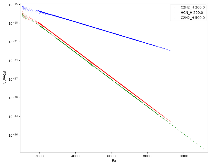
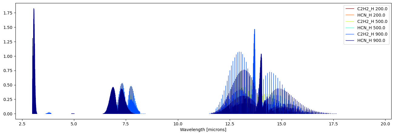
4.1. Plotting Boltzmann diagram
plotBoltzmannDiagram(data,ax=None,fig=None,figsize=None,NLTE=False,label=None,s=0.1,c=’k’,set_axis_limits=True)
[21]:
fig,ax = ps.plotBoltzmannDiagram(data[0:3],
                                 c=['r','g','b'],
                                 label=[d.species_name+' '+str(d.Tg) for d in data[0:3]],
                                 figsize=(10,8))
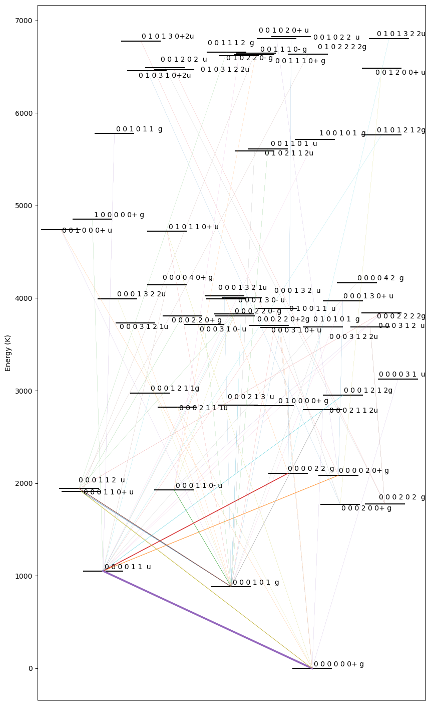
4.2. Plotting energy level diagram
plotLevelDiagram(data,ax=None,figsize=(10,18),seed=None,lambda_0=None,lambda_n=None,width_nlines=False):
This function takes in only 1 slab model at a time. The arrangement of the levels along the x axis is random, hence the function also returns the seed used to generate it (also prints). The seed can be passed as an argument to retrieve the same arrangement of levels again. The thickness of the line is proportional to the total flux that band is contributing. width_nlines can be set to True to make the line thickness proportional to the number of lines in that band. lambda_0 and lambda_n can be used to focus on certain spectral region to make the level diagram. This can be helpful to analyse which bands are contributing to a certain spectral feature.
[22]:
fig,ax,seed = ps.plotLevelDiagram(data[2]) # try this seed 7153029
Random seed = 7872905
4.3. Plotting the line fluxes
plot_lines(dat, normalise = False, fig=None, ax=None, overplot=False, c=None, cmap=None, colors=None, figsize=None, NLTE=False, label=’’, lw=1, scaling=1,offset=0):
Not passing any figure or axis objects will generate one figure and one axis object per slab model. This will be returned in two separate lists. normalise argument can be used to normalise the fluxes with peak flux. scaling argument can be used to scale the fluxes by any factor. Since it is a numpy multiplication, it can support either scalars or arrays of same size as number of lines offset argument can be used to offset the fluxes. Since it is a numpy multiplication, it can support either scalars or arrays of same size as number of lines. This can be useful for adding a background/continuum.
The colors can be specified as a single color c or list of colors with the argument colors or can as well pass the name of a color map (by default it uses ‘jet’ colormap for single figure and black color for separate figures)
NOTE: the Y axis of all the plots containing line fluxes and line spectra are in units [erg/s/cm2/sr] when not scaled or normalised
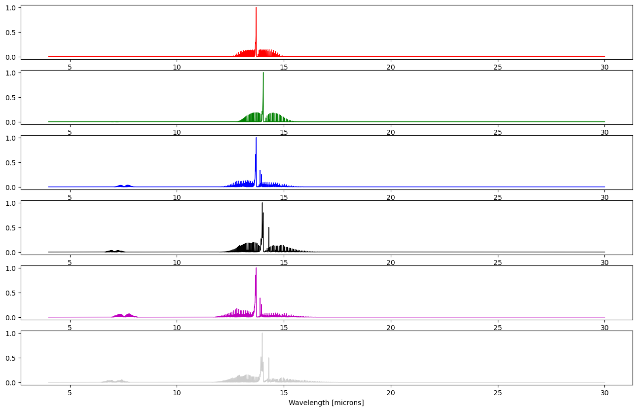
4.3.1. Plotting the line fluxes in separate figures
This can be done in two ways. First way to simply call the plotting function and pass the slab models. For example: [fig_array,ax_array] = ps.plot_lines(data,label=[d.species_name+’ ‘+str(d.Tg) for d in data]) This returns two arrays containing figures and axis objects respectively. Second way is to generate the figure and axes objects using matplotlib pyplot subplots and passing that to the function. For example: fig,ax = plt.subplots(data.nmodels,1) ps.plot_lines(data,fig=fig,ax=ax,label=[d.species_name+’ ‘+str(d.Tg) for d in data]);
[23]:
fig,ax = plt.subplots(data.nmodels,1,figsize=(16,10))
ps.plot_lines(data,
              fig=fig,
              ax=ax,
              label=[d.species_name+' '+str(d.Tg) for d in data],
              colors=['r','g','b','k','m','0.8']);
4.3.2. Plotting the line fluxes in single figure
This can be done in two ways. First way to pass overplot=True argument to the plotting function along with the slab models. For example: fig,ax = ps.plot_lines(data,label=[d.species_name+’ ‘+str(d.Tg) for d in data],overplot=True) This returns the figure and axis objects respectively. Second way is to generate the figure and axes objects using matplotlib pyplot subplots and passing that to the function. For example: fig,ax = plt.subplots(1,1) ps.plot_lines(data,fig=fig,ax=ax,label=[d.species_name+’ ‘+str(d.Tg) for d in data]);
[24]:
fig,ax = ps.plot_lines(data,
                       label=[d.species_name+' '+str(d.Tg) for d in data],
                       overplot=True,
                       cmap='jet_r')
4.4. Plotting the spectra
plot_spectra(dat, normalise = False, fig=None, ax=None, overplot=False, add=False, cmap=None, colors=None, style=’step’, figsize=None, NLTE=False, label=’’, lw=1, c=None, scaling=1,sampling=1,offset=0): To plot the spectra, the slab models have to first be convolved at a spectral resolving power by the user. See Sect. 3.
scaling, offset and normalise can be used to scale, offset and normalise the spectra. Like explained before, scaling and offset can be scalar or numpy arrays of size same as that of the convolved grid.
add=True can be used to add up the individual slab spectra to produce a composite slab spectra. See Sect 4.4.3.
The oversampling can be specified by sampling argument which is 1 by default.
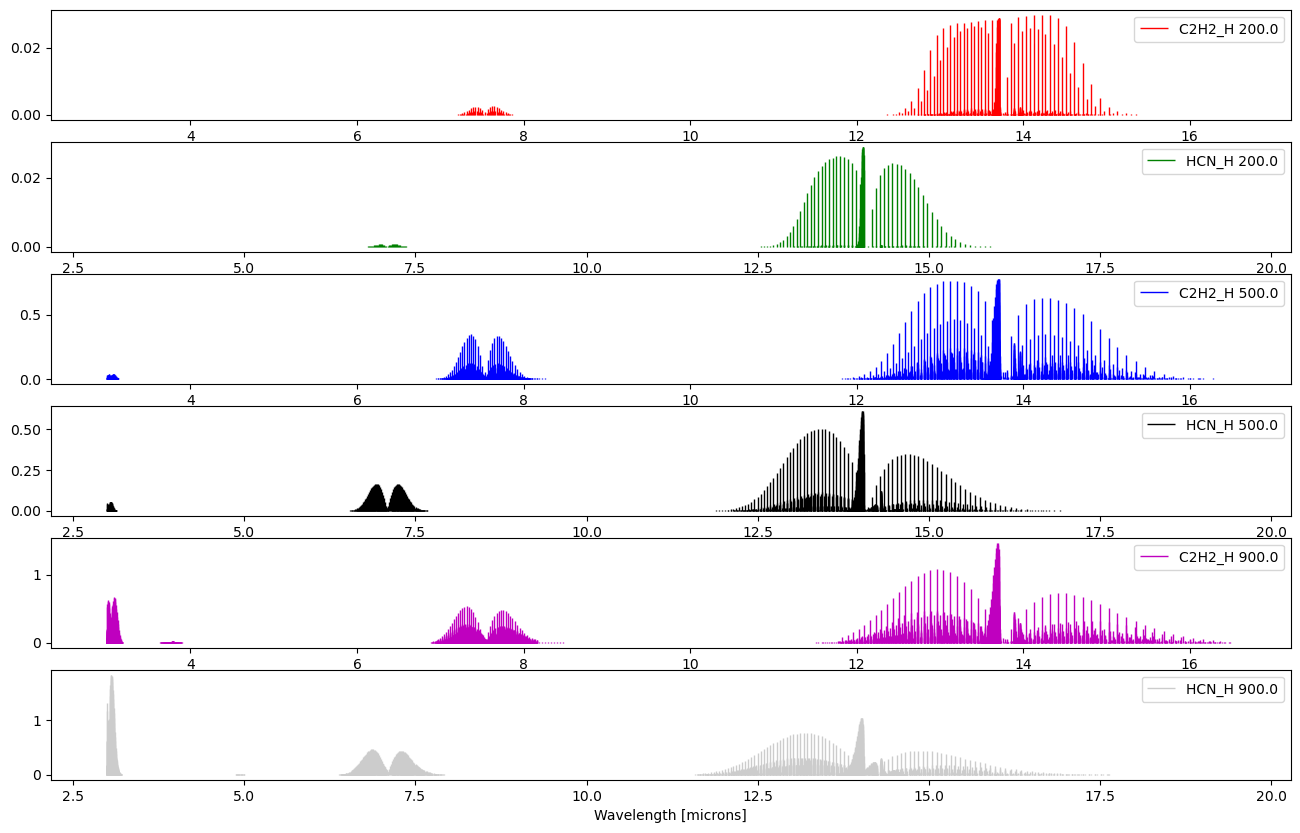
4.4.1. Plotting the spectra in separate figures
This can be done in two ways. First way to simply call the plotting function and pass the slab models. For example: [fig_array,ax_array] = ps.plot_spectra(data,label=[d.species_name+’ ‘+str(d.Tg) for d in data]) This returns two arrays containing figures and axis objects respectively. Second way is to generate the figure and axes objects using matplotlib pyplot subplots and passing that to the function. For example: fig,ax = plt.subplots(data.nmodels,1) ps.plot_spectra(data,fig=fig,ax=ax,label=[d.species_name+’ ‘+str(d.Tg) for d in data]);
[25]:
fig,ax = plt.subplots(data.nmodels,1,figsize=(16,10))
ps.plot_spectra(data,
                fig=fig,
                ax=ax,
                label=[d.species_name+' '+str(d.Tg) for d in data],
                colors=['r','g','b','k','m','0.8'],
                normalise=True);
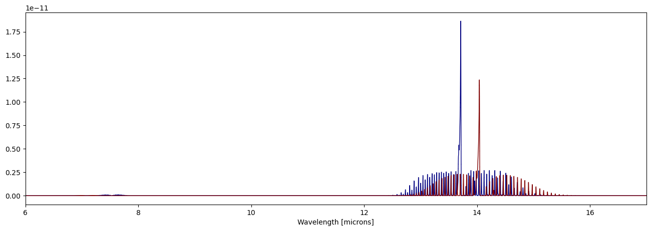
4.4.2. Plotting the spectra in single figure
This can be done in two ways. First way to pass overplot=True argument to the plotting function along with the slab models. For example: fig,ax = ps.plot_spectra(data,label=[d.species_name+’ ‘+str(d.Tg) for d in data],overplot=True) This returns the figure and axis objects respectively. Second way is to generate the figure and axes objects using matplotlib pyplot subplots and passing that to the function. For example: fig,ax = plt.subplots(1,1) ps.plot_spectra(data,fig=fig,ax=ax,label=[d.species_name+’ ‘+str(d.Tg) for d in data]);
[26]:
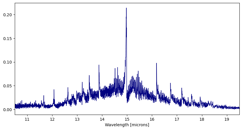
fig,ax = ps.plot_spectra(data['Tg':200],
                         overplot=True,
                         label=[d.species_name[:-2]+'@'+str(d.Tg)+'K' for d in data['Tg':200]],
                         figsize=(16,5))
ax.set_xlim([6,17])
[26]:
(6.0, 17.0)
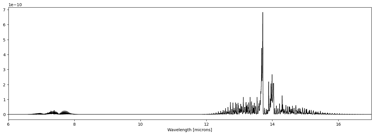
4.4.3. Plotting the combined spectra of multiple slab models
add=True can be used to add up the individual slab spectra to produce a composite slab spectra.
[27]:
fig,ax = ps.plot_spectra(data['Tg':500],
                         add=True,
                         label='Combined spectra at 500K',
                         figsize=(16,5),
                         sampling=2)
ax.set_xlim([6,17]);
5. Reading the HITRAN data
Data files from HITRAN database can be read using prodimopy.hitran read_hitran(filePath, moleculeName, isotopologue:list=[1], lowerLam:int=1, higherLam:int=30, sort_label=’lambda’, quanta=False, format:int=2020, verbose:bool=False) Older formats of HITRAN can be read by changing the format argument. The default is 2020.
The quantum numbers of the upper and lower global and local levels can also be decoded using quanta=True argument. However, this may fail for some molecules.
The read data is returned in a Pandas DataFrame
[28]:
file = '/home/rab/git/prodimo/data/HITRAN2020/C2H2.par'
hit_data = ht.read_hitran(file,moleculeName='C2H2')
hit_data
/home/rab/git/prodimopy/prodimopy/hitran.py:503: FutureWarning: Downcasting object dtype arrays on .fillna, .ffill, .bfill is deprecated and will change in a future version. Call result.infer_objects(copy=False) instead. To opt-in to the future behavior, set `pd.set_option('future.no_silent_downcasting', True)`
  data['line_mixing']=data['line_mixing'].fillna(False)
[28]:
| Molecule_ID | Isotopologue_ID | lambda | nu | S | A | gamma_air | gamma_self | E_u | E_l | ... | del_air | global_u | global_l | local_u | local_l | err_ind | References | line_mixing | g_u | g_l | |
|---|---|---|---|---|---|---|---|---|---|---|---|---|---|---|---|---|---|---|---|---|---|
| 83436 | 26 | 1 | 1.003637 | 9963.76240 | 9.871000e-27 | 0.000546 | 0.0524 | 0.098 | 10918.12720 | 954.3648 | ... | -0.001 | 111 0 2 0 0+ u | 000 0 0 0 0+ g | NaN | R 28e | 356643 | 2219 2 1 1 1 | False | 59.0 | 57.0 |
| 83435 | 26 | 1 | 1.003766 | 9962.47770 | 3.929000e-26 | 0.000545 | 0.0541 | 0.101 | 10851.09300 | 888.6153 | ... | -0.001 | 111 0 2 0 0+ u | 000 0 0 0 0+ g | NaN | R 27e | 356643 | 2219 2 1 1 1 | False | 171.0 | 165.0 |
| 83434 | 26 | 1 | 1.003901 | 9961.14370 | 1.716000e-26 | 0.000543 | 0.0560 | 0.104 | 10786.34810 | 825.2044 | ... | -0.001 | 111 0 2 0 0+ u | 000 0 0 0 0+ g | NaN | R 26e | 356643 | 2219 2 1 1 1 | False | 55.0 | 53.0 |
| 83433 | 26 | 1 | 1.004040 | 9959.76120 | 6.657000e-26 | 0.000542 | 0.0578 | 0.107 | 10723.89420 | 764.1330 | ... | -0.001 | 111 0 2 0 0+ u | 000 0 0 0 0+ g | NaN | R 25e | 356643 | 2219 2 1 1 1 | False | 159.0 | 153.0 |
| 83432 | 26 | 1 | 1.004077 | 9959.39620 | 8.536000e-27 | 0.000036 | 0.0733 | 0.132 | 10279.32360 | 319.9274 | ... | -0.001 | 130 0 1 0 1 u | 000 0 0 0 0+ g | NaN | R 16e | 356643 | 2219 2 1 1 1 | False | 35.0 | 33.0 |
| ... | ... | ... | ... | ... | ... | ... | ... | ... | ... | ... | ... | ... | ... | ... | ... | ... | ... | ... | ... | ... | ... |
| 5523 | 26 | 1 | 25.165840 | 397.36404 | 3.665000e-28 | 0.000278 | 0.0450 | 0.081 | 3254.21434 | 2856.8503 | ... | -0.001 | 000 2 0 2 0 g | 000 0 1 0 1 u | NaN | P 42f | 345543 | 2320 2 1 1 1 | False | 83.0 | 85.0 |
| 5522 | 26 | 1 | 25.325368 | 394.86100 | 6.886000e-28 | 0.000275 | 0.0450 | 0.081 | 3352.75900 | 2957.8980 | ... | -0.001 | 000 2 0 2 0 g | 000 0 1 0 1 u | NaN | P 43f | 345543 | 2320 2 1 1 1 | False | 255.0 | 261.0 |
| 5521 | 26 | 1 | 25.460632 | 392.76322 | 1.511000e-28 | 0.000092 | 0.0450 | 0.081 | 3444.88402 | 3052.1208 | ... | -0.001 | 000 2 0 2 0 g | 000 0 1 0 1 u | NaN | P 44e | 345543 | 2320 2 1 1 1 | False | 261.0 | 267.0 |
| 5520 | 26 | 1 | 25.487112 | 392.35516 | 1.420000e-28 | 0.000272 | 0.0450 | 0.081 | 3453.62536 | 3061.2702 | ... | -0.001 | 000 2 0 2 0 g | 000 0 1 0 1 u | NaN | P 44f | 345543 | 2320 2 1 1 1 | False | 87.0 | 89.0 |
| 5519 | 26 | 1 | 25.651120 | 389.84653 | 2.606000e-28 | 0.000269 | 0.0450 | 0.081 | 3556.81153 | 3166.9650 | ... | -0.001 | 000 2 0 2 0 g | 000 0 1 0 1 u | NaN | P 45f | 345543 | 2320 2 1 1 1 | False | 267.0 | 273.0 |
68326 rows × 21 columns
The level format can be retrieved using getLevelFormat(molecule:str,format:int=2020,level:str=’global’)
[29]:
ht.getLevelFormat('CO2',
                  format=2020,
                  level='global')
[29]:
'v1 v2 l2 v3 r '
[30]:
ht.getLevelFormat('CO2',
                  format=2020,
                  level='local')
[30]:
'm F '
[31]:
ht.getLevelFormat('CO2',
                  format=2009,
                  level='local')
[31]:
'F '
6. Generating SlabInput.in file for a ProDiMo slab run
generate_slab_grid(directory=’.’, grid_parameters={}, combination=False, Ntot=None, Tg=None, nHplus=None, nH1=None, nH2=None, nHe=None, nelec=None, Td=None, vturb=None, dust_to_gas=None, species_list={}, output_filename=’SlabResults.out’, separate_op_files=True)
Argument | Datatype | Description | Default value |
|---|---|---|---|
directory | string | directory where the SlabInput.in file is to be created | ‘.’ |
grid_parameters | dict | Dictionary containing the varying grid parameters. Each parameter should be associated with the list of values corresponding to each slab model. The length of such lists for each grid parameter should be the same | {} |
combination | logical | Under development | False |
Ntot | int or float | The default value of gas column density across models | 1e15 |
Tg | int or float | The default value of gas temperature across models | 100 |
nHplus | int or float | The default value of H+ number density across models | 1e1 |
nH1 | int or float | The default value of atomic hydrogen number density across models | 1e12 |
nH2 | int or float | The default value of molecular hydrogen number density across models | 1e12 |
nHe | int or float | The default value of Helium number density across models | 1e11 |
nelec | int or float | The default value of electron number density across models | 1e8 |
Td | int or float | The default value of dust temperature across models | 10 |
vturb | int or float | The default value of gas turbulent velocity across models | 1.4 |
dust_to_gas | int or float | The default value of dust to gas ratio across models | 1e-21 |
species_list | dict | Dictionary containing molecule names as keys and their abundance as values. Cannot be empty | {} |
output_filename | string | Filename for storing the output of slab models. To include the directory use the following format: f‘“folder/filename”’ | None |
separate_op_files | logical | If true, one file per slab model is generated. The name of each file is output_filename followed by a number with leading zeros. | False |
Note: The column density of the spiecies is given by total gas column denisty times the species abundance (Ntot x species_abundance)
The following example produces the SlabInput.in file used in the example output file in this notebook
[33]:
parameter_space = {'Tg':[200,500,900]}
rs.generate_slab_grid(directory       = '.',
                      grid_parameters = parameter_space,
                      species_list    = {'C2H2_H':0.001,
                                         'HCN_H':0.001},
                      Ntot=1e19,
                      separate_op_files=False,)
The following generates a 2x2 grid for gas temperature and total gas column density.
[34]:
parameter_space = {'Tg':[100,200,100,200],'Ntot':[1e16,1e16,1e20,1e20]}
rs.generate_slab_grid(directory       = '.',
                      grid_parameters = parameter_space,
                      species_list    = {'C2H2_H':0.001,
                                         'HCN_H':0.001},
                      Ntot=1e19,
                      separate_op_files=False,)
7. Models with opacity overlap
7.1. Running the models
Visit readthedocs for more information:
Models with line opacity overlap are output in a different format. These models can be run via ProDiMo or with prodimopy. Check ProDiMo wiki for more info on how to run these models on ProDiMo FORTRAN package. The run commands/functions for prodimopy are available via prodimopy.run_slab, however are limited to one molecule per model only. To run the 0D opacity overlap slab models on python the following command can be used:run_0D_slab(Ng, Tg, vturb, molecule, mol_mass, HITRANfile, R_grid, QTpath, output_filename, isotopolog=[1], wave_mol=[4, 30], wave_spec=[4.9, 28])
Information about what goes into each argument can be found with help(run_0D_slab).
[35]:
help(runs.run_0D_slab)
Help on function run_0D_slab in module prodimopy.run_slab:

run_0D_slab(Ng, Tg, vturb, molecule, mol_mass, HITRANfile, QTpath, isotopolog=[1], wave_mol=[4, 30], wave_spec=[4.9, 28], R_grid=100000.0, output='both', output_filename='default.out', mode='both', verbose=True)
    This is a python implementation of 0D slab models, based on the FORTRAN version of 0D slab models in ProDiMo (https://prodimo.iwf.oeaw.ac.at/)
    This runs models with/without line overlap. More robust and efficient code is available on Fortran, please check the above website (especially for running large grids of models).
    The Fortran code also supports OMP and supports including multiple species.

    Ng : float
        Gas column density (cm-2)

    Tg: float
        Gas temperature (K)

    vturb : float
        Turbulent velocity of the gas (km/s)

    molecule : string
        Molecule name, e.g. 'CO2'

    mol_mass : float or int
        Molecular mass in atomic mass units (amu)

    HITRANfile : string
        Path to the HITRAN '.par' file containing the line data downloaded from HITRAN

    QTpath : string
        Path pointing to directory containing the directory QTpy provided by HITRAN (see hitran.org)

    output_filename: string
        Filename(+path) for the fits output file
        Use the extension '.fits.gz'

    isotopolog : list
        List containing isotopologue numbers (HITRAN format)

    wave_mol : list
        Wavelength limits in microns to select the lines from the HITRAN file

    wave_spec : list
        Wavelength limits in microns for calculating the spectra

    R_grid : float
        High resolution grid on which the spectra has to be calculated initially
        Recommend minimum of 1e5

    overlap : boolean
        Whether or not to perform line overlap calculations

    verbose : boolean
        Whether or not to print progress log
The following demonstrates running a slab model with opacity overlap with parameters: gas column density = 1e18cm-2, gas temperature = 250K, turbulent velocity = 2km/s, species = CO2, molecular mass = 44 amu, HITRAN file of CO2 located at ‘path/to/file.par’, spectral resolving power = 1e5, path to directory containing the QTpy directory = ‘path/to/directory/’, output file = ‘CO2.fits.gz’, with spectral limits of 4-30 microns.
[36]:
runs.run_0D_slab(Ng              = 1e18,
                 Tg              = 250,
                 vturb           = 2,
                 molecule        = 'CO2',
                 mol_mass        = 44,
                 HITRANfile      = '/home/rab/git/prodimo/data/HITRAN2020/CO2.par',
                 R_grid          = 1e5,
                 QTpath          = '/home/rab/MODELS/HITRANTIPS/TIPS_2021_PYTHON/QTpy/',
                 output_filename = 'CO2',
                 isotopolog      = [1],
                 wave_mol        = [4,30],
                 wave_spec       = [4.9,28])
/home/rab/git/prodimopy/prodimopy/hitran.py:503: FutureWarning: Downcasting object dtype arrays on .fillna, .ffill, .bfill is deprecated and will change in a future version. Call result.infer_objects(copy=False) instead. To opt-in to the future behavior, set `pd.set_option('future.no_silent_downcasting', True)`
  data['line_mixing']=data['line_mixing'].fillna(False)
Output written to CO2.fits.gz
Output written to CO2.out
[36]:
<prodimopy.read_slab.slab_data at 0x154bd4bc72f0>
This produces a fits output file containing the column of frequency, flux and opacity. The speed on python is low, typically ~20 times slower than on FORTRAN.
7.2. Running 1D slab models
1D models are implemented in ProDiMo FORTRAN package. These models are vertical slab models, see ProDiMo wiki for more information on the code implementation and assumptions. However these can be converted into a horizontal/radial slab model with ease, shown later.
However, 1D radial models can be run also on python using prodimopy, with the same limitation of only one molecule and no dust opacity. This can be run with:run_1D_radial_slab(Ng, Tg, R, d, vturb, molecule, mol_mass, HITRANfile, R_grid, QTpath, output_filename, width=’area_given’, Rin_limit=0, Rout_limit=1e99, isotopolog=[1], wave_mol=[4,30], wave_spec=[4.9,28]) The description of arguments can be found by help command.
[37]:
help(runs.run_1D_radial_slab)
Help on function run_1D_radial_slab in module prodimopy.run_slab:

run_1D_radial_slab(Ng, Tg, R, d, vturb, molecule, mol_mass, HITRANfile, R_grid, QTpath, output_filename, width='area_given', Rin_limit=0, Rout_limit=1e+99, isotopolog=[1], wave_mol=[4, 30], wave_spec=[4.9, 28], verbose=False)
    This is a python implementation of 1D radial slab models, based on the FORTRAN version of 1D slab models in ProDiMo (https://prodimo.iwf.oeaw.ac.at/)
    This runs models with line overlap. More robust and efficient code (including vertical slab model) is available in Fortran, please check the above website (especially for running large grids of models).
    The Fortran code also supports OMP and supports including multiple species.

    Ng : numpy array or list
        Gas column density (cm-2)

    Tg : numpy array or list
        Gas temperature (K)

    R : numpy array or list
        Radius (AU)

    d : float
        Distance of the disk (parsec)

    vturb : float
        Turbulent velocity of the gas (km/s)

    molecule : string
        Molecule name, e.g. 'CO2'

    mol_mass : float or int
        Molecular mass in atomic mass units (amu)

    HITRANfile : string
        Path to the HITRAN '.par' file containing the line data downloaded from HITRAN

    R_grid : float
        High resolution grid on which the spectra has to be calculated initially
        Recommend minimum of 1e5

    QTpath : string
        Path pointing to directory containing the directory QTpy provided by HITRAN (see hitran.org)

    output_filename : string
        Filename(+path) for the fits output file
        Use the extension '.fits.gz'

    width : string or list or float
        'area_given' - the provided radii array is used as the emitting area equivalent radius
        'infer' - Assumes the provided radius as radial distance from the star and calculates the width of individual rings of slab grids
        list - List containing emitting area equivalent radii
        float - Constant emitting area equivalent radius, used for all grid points

    Rin_limit : float
        Inner radius limit of the disk (AU)

    Rout_limit : float
        Outer radius limit of the disk (AU)

    isotopolog : list
        List containing isotopologue numbers (HITRAN format)

    wave_mol : list
        Wavelength limits in microns to select the lines from the HITRAN file

    wave_spec : list
        Wavelength limits in microns for calculating the spectra
The following shows an example of running a radial slab with 5 grid points.
[38]:
runs.run_1D_radial_slab(Ng              = [1e22,1e21,1e20,1e19,1e18],
                        Tg              = [ 650, 450, 350, 300, 250],
                        R               = [0.07, 0.1,0.15, 0.2, 0.5],
                        d               = 190,
                        vturb           = 2,
                        molecule        = 'CO2',
                        mol_mass        = 44,
                        HITRANfile      = '/home/rab/git/prodimo/data/HITRAN2020/CO2.par',
                        R_grid          = 1e5,
                        QTpath          = '/home/rab/MODELS/HITRANTIPS/TIPS_2021_PYTHON/QTpy/',
                        output_filename = 'CO2_1D',
                        width           = 'infer',
                        isotopolog      = [1],
                        wave_mol        = [4,30],
                        wave_spec       = [4.9,28])
/home/rab/git/prodimopy/prodimopy/hitran.py:503: FutureWarning: Downcasting object dtype arrays on .fillna, .ffill, .bfill is deprecated and will change in a future version. Call result.infer_objects(copy=False) instead. To opt-in to the future behavior, set `pd.set_option('future.no_silent_downcasting', True)`
  data['line_mixing']=data['line_mixing'].fillna(False)
Note that the computation speed of the model is very low, if large number of models are to be run, e.g. a grid, then running models with the FORTRAN version is highly recommended.
7.3. Reading the models
The model outputs can be read using the prodimopy.read_slab functions. The overlap 0D slab model can be read using the read_slab function that was introduced above, but need to pass overlap_model=True. Note that these models have minimum data in the output, so many features of prodimopy described above might be limited.
[40]:
CO2_0D = rs.read_slab('CO2.fits.gz')
Reading slab line overlap model output from: CO2.fits.gz
1D ProDiMo FORTRAN models can be read using read_1D_slab function. However, the python implementation is very trivial and does not store the source functions, optical depths, etc of individual grids, instead outputs a single spectra similar to the above overlap 0D slab models. Hence, the output format is also the same as the 0D overlap slab model.
[42]:
CO2_1D = rs.read_slab('CO2_1D.fits.gz')
Reading slab line overlap model output from: CO2_1D.fits.gz
[43]:
CO2_0D.convolve(R=3000,lambda_0=4,lambda_n=30,overlap=True)
CO2_1D.convolve(R=3000,lambda_0=4,lambda_n=30,overlap=True)
 1 ; Model number  1 ; Species number  None

 1 ; Model number  1 ; Species number  None
[44]:
[(fig,ax)] = ps.plot_spectra(CO2_0D,overlap=True)
ax.set_xlim([12.5,17.5])
[44]:
(12.5, 17.5)
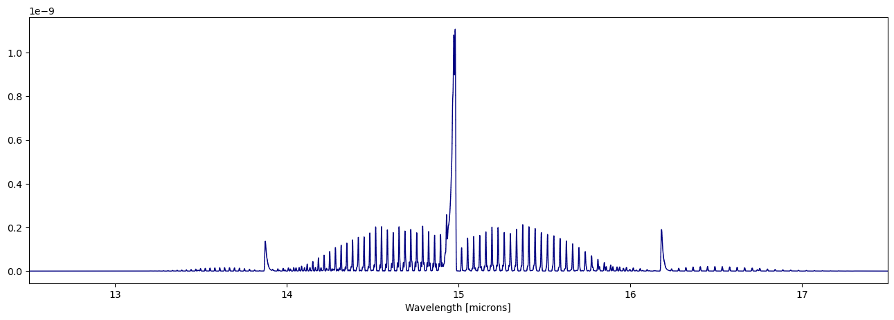
[45]:
jansky = 1e23
fig,ax = plt.subplots(figsize=(10,5))
ps.plot_spectra(CO2_1D,overlap=True,scaling=jansky,fig=fig,ax=ax)
ax.set_xlim([10.5,19.5])
[45]:
(10.5, 19.5)