Setting up and plotting a dynamic MC model

This notebook shows how to set up and plot a dynamic molecular cloud model. Dynamic means that the physical conditions change with time. In this example we change the UV field with time to simulate an accretion bursts. The notebook shows how to generate the required input file mc_dynamic.in and example of how to plot the results using prodimopy.

Initial steps

At first we need to copy the initial ProDiMo setup for this example. These can be found within your prodimo installation in the folder examples/MolecularCloud/mc_dynamic. Just copy the mc_dynamic folder (which contains two models) to a working directory of your choice
Download this notebook to this mc_dynamic folder you have just copied and then open it with jupyter notebook or vscode.

[5]:

import prodimopy.read_mc as preadmc
import prodimopy.plot_mc as pplotmc
import numpy as np
import copy
import prodimopy.plot as pplot
pplot.load_style("nb")

INFO: Load prodimopynb mplstyle from package.

Setting the default physical conditions

At first we have to define our default physical conditions, i.e. the physical conditions that will be used for the model at all times, except for the times where we will have the burst.

[6]:

# Setting the default physical conditions
# we use the MCParameterSet class of prodimopy to do that.
# This also shows what parameters change be changed as function of time in a dynamic molecular cloud prodimo model.
pdef = preadmc.MCParameterSet()
pdef.nH = 1.0e8
pdef.td = 250.0
pdef.tg = 250.0
pdef.CHI1 = 1.0e4
pdef.CHI2 = 1.0e4
pdef.a1 = 0.1
pdef.dust_to_gas = 0.001
pdef.rho_gr = 3.0
pdef.vturb = 1.0
pdef.CRI = 1.3e-17
pdef.Av = 1.0
pdef.albedo = 0.5

Create the input file for the dynamic model

[7]:

# At first we need a time grid, i.e. age of the 0D molecular cloud model.

# just let it evolve for 1 Myr, to reach a steady state
ages = np.logspace(-2, np.log10(1e6), 20)

# now add linear timesteps this will be the times where we change something, we add 20 points from 1 Myr +10 years to 1 Myr + 200 years, to simulate an accretion burst
agesburst = ages[-1] + np.linspace(10, 200, 20)
ages = np.append(ages, agesburst)

# now let it evolve for another 1 Myr after the burst
agespostburst = ages[-1] + np.logspace(-3, np.log10(1e6), 50)
ages = np.append(ages, agespostburst)

# we copy the parameter set for each age, so that we make sure that the parameters that do not change are the same
params = [copy.deepcopy(pdef) for age in ages]

# now we write the input file for a reference model that does not have a burst, but we still use the mc_dynamic.in format. This makes it easier to compare the model results
preadmc.write_mc_dynamic_input(ages, params, filename="MCDYN_REF/mc_dynamic.in")

# now we change some parameters for the burst
# keep some points before and after the burst unchanged, will look nicer for plotting
# so the burst duration will be 100 years
maskburst = (ages > (1e6) + 50) & (ages < 1e6 + 150)
for paramset in np.array(params)[maskburst]:
    paramset.CHI1 = 1.0e6
    paramset.CHI2 = 1.0e6

# write the file the for the burst model
preadmc.write_mc_dynamic_input(ages, params, filename="MCDYN_BURST/mc_dynamic.in")

INFO: Writing dynamic model input to file:  MCDYN_REF/mc_dynamic.in  ...
INFO: Writing dynamic model input to file:  MCDYN_BURST/mc_dynamic.in  ...

Run the models

We assume you already have prodimo running and you also have prodimopy installed.

To run the model change into the MCDYN_REF folder and type ‘prunprodimo’ in the terminal. This will run the reference model without the burst. After that, change into the MCDYN_BURST folder and run ‘prunprodimo’ there to run the model with the burst.

When the models are finished (check the prodimo.log files) we can start plotting the results.

Plot the results

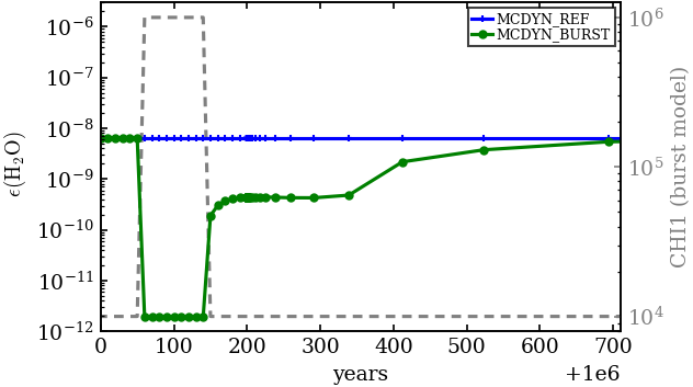
In the following figure we compare the model without the burst and the model with the burst. As it can be seen, it takes some time after the burst until the chemistry reaches again the same steady-state as the model without the burst.

[8]:

# Now we compare those two models
mref = preadmc.read_mc("MCDYN_REF")
mburst = preadmc.read_mc("MCDYN_BURST")

pp = pplotmc.PlotMcModels(markers=["+", "o"])

fig = pp.plot_species(
    [mref, mburst],
    "H2O",
    labels=["reference", "burst"],
    xlim=[1.0e6, 1e6 + 710], # we zoom in on the burst
    ylim=[1.0e-12, 3.0e-6],
    xlog=False,
    ms=3,
)

# now we add the second axis to show the change of the CHI parameter
ax = fig.axes[0]
ax2 = ax.twinx()
ax.patch.set_alpha(0.0)
ax2.set_zorder(ax.get_zorder() - 1)
ax2.plot(
    mref.ages,
    [x.CHI1 for x in mburst.physicalParameters],
    color="0.5",
    linestyle="--",
)
ax2.semilogy()
ax2.tick_params(axis="y", colors="0.5")
ax2.set_ylabel("CHI1 (burst model)", color="0.5")

INFO: Reading dynamic model ...
READ: Reading File:  MCDYN_REF/mc_species.txt  ...
READ: Reading File:  MCDYN_REF/mc_ages_001.txt  ...
READ: Reading File:  MCDYN_REF/mc_output_001.out  ...
INFO: Reading dynamic model ...
READ: Reading File:  MCDYN_BURST/mc_species.txt  ...
READ: Reading File:  MCDYN_BURST/mc_ages_001.txt  ...
READ: Reading File:  MCDYN_BURST/mc_output_001.out  ...

[8]:

Text(0, 0.5, 'CHI1 (burst model)')