ProDiMo 2D interface
[14]:
import os

import numpy as np
import astropy.units as u

import h5py as h5

import prodimopy.interface2D.infile as pin2D
import prodimopy.plot as pplot
import prodimopy.read as pread
import prodimopy.plot_models as pplotm
import matplotlib.pyplot as plt

# load the default style for the plots
pplot.load_style()
plt.rcParams['figure.dpi'] = 100 # set the resolution of the plots, useful to scale the figure size in a notebook
INFO: Load prodimopy mplstyle from package.
Utility routines for reading the MHD files
This model is from the Nirvana code (Used in this paper https://ui.adsabs.harvard.edu/abs/2025arXiv251102811W). Usually such routines need to be developed for each type of Hydro model. This has to be done by the user, we do not provide routines for any particular (M)HD code. But it might be worth asking the ProDiMo community (e.g. on slack) if somebody has already used the 2D interface for your type of (M)HD model.
[15]:
def iterative_mean(dat, t, mean=None):
    """
    Compute the iterative mean of data arrays.
    """
    if mean is None:
        mean = np.zeros(dat.shape)
    mean += 1.0 / (t + 1) * (dat - mean)

    return mean


def cart2pol(x, y):
    """
    Conversion of the coordinate system to cartesian. Done in the same way as Michael did.
    """
    r = np.sqrt(x**2 + y**2)
    theta = np.arccos(y / r)
    return (r, theta)


def vpol2cart(vr, vt, x, y):
    """
    Convert velocity components from polar to cartesian coordinates.
    """
    r, theta = cart2pol(x, y)
    sint = np.sin(theta)
    cost = np.cos(theta)
    vx = vr * sint + vt * cost
    vy = vr * cost - vt * sint

    return (vx, vy)


def load_mhdmodel(mdir):
    """
    Load the MHD model from a directory containing multiple h5 files
    and average them to get a time-averaged model.

    Returns a prodimopy Interface2Din object.
    """

    # For converting code units to real units
    UNIT_LENGTH = 1 * u.au
    UNIT_DENSITY = 1 * u.M_sun / u.au**3
    UNIT_VELOCITY = 2.978e4 * u.m / u.s

    if mdir.startswith("~"):
        mdir = os.path.expanduser(mdir)

    h5files = os.listdir(mdir)

    density = None
    velocity = None
    temperature = None
    i = 0
    for fname in h5files:
        if not fname.endswith(".h5"):
            continue
        try:
            with h5.File(os.path.join(mdir, fname), "r") as f:
                if density is None:
                    # This would print all available keys in the h5 file
                    #print(*f.keys(),sep="\n")
                    x = np.array(f["_x"])
                    y = np.array(f["_y"])
                    z = np.array(f["_z"])
                density = iterative_mean(np.array(f["density"]), i, density)
                velocity = iterative_mean(np.array(f["velocity"]), i, velocity)
                temperature = iterative_mean(np.array(f["temperature"]), i, temperature)
                i += 1
            f.close()
        except Exception as e:
            print("could not read", fname, "due to", e)

    # velocity is in vr,vtheta,vphi
    # get vx and vz from vr and
    vy = velocity[:, :, 2]
    vx, vz = vpol2cart(velocity[:, :, 0], velocity[:, :, 1], x, z)

    velocity[:, :, 0] = vx
    velocity[:, :, 1] = vy
    velocity[:, :, 2] = vz

    # flip so that z=0 has zidx=0
    x = np.flip(x, 1)
    z = np.flip(z, 1)
    density = np.flip(density, 1)
    velocity = np.flip(velocity, 1)
    temperature = np.flip(temperature, 1)

    # It seems that z can be < 0 in the midplane ... set it to zero
    z[z[:, 0] < 0, 0] = 0.0

    # Use the prodimopy tools to generate an object for further processing
    return pin2D.Interface2Din(
        ((x * UNIT_LENGTH).to(u.cm)).value,
        ((z * UNIT_LENGTH).to(u.cm)).value,
        rhoGas=((density * UNIT_DENSITY).to(u.g / u.cm**3)).value,
        velocity=((velocity * UNIT_VELOCITY).to(u.cm / u.s)).value,
        tgas=temperature,
    )
Load the MHD model
Here wie load the MHD model creating a snapshot of a couple of time-steps. Furthermore we manipulate the data to get rid of some unphysical values.
[16]:
# load the MHD model
mhd2DIn = load_mhdmodel("~/MODELS/prodimopy/dfl-10_b4")

# Make some manipulations
# remove everything inside the inner boundary of the model
xxnew = (mhd2DIn.x * u.cm).to(u.au).value
zznew = (mhd2DIn.z * u.cm).to(u.au).value
rrnew = np.sqrt(xxnew**2 + zznew**2)
rincut = rrnew.min() * 0.95  # use this as the cut ...

MU = 1.37
print("muH=", (MU * u.M_p).cgs)
vzcart = mhd2DIn.velocity[:, :, 2]
nhcart = mhd2DIn.rhoGas[:, :] / (MU * ((1.0 * u.M_p).cgs))
mask_infall = np.zeros_like(xxnew, dtype=bool)
mask_infall = (xxnew < rincut) | (nhcart.cgs.value < 6e4)

def fcut(x):
    return x * 7 + 0.5

# get rid of the rest of the infall
# cut some residual stuff
for ix in range(len(xxnew[:, 0])):
    mask_infall[ix, :] = mask_infall[ix, :] | (zznew[ix, :] > fcut(xxnew[ix, :]))

mhd2DIn.velocity[(xxnew < rincut * 1.5) & (mhd2DIn.velocity[:, :, 0] < 0.0), 0] = 0.0
mhd2DIn.velocity[(xxnew < rincut * 1.5) & (mhd2DIn.velocity[:, :, 2] < 0.0), 2] = 0.0
nhcart[mask_infall] = np.nan

mhd2DIn.rhoGas[mask_infall] = np.nan
for i in range(3):
    mhd2DIn.velocity[mask_infall, i] = np.nan

# get a prodimopy representation for this model for plotting
# This provides a prodimopy.read.Data_ProDiMo object, which is convenient for plotting
mhdpmodel = mhd2DIn.get_pmodel()
muH= 2.2914920354553003e-24 g
Plotting the MHD model
With the prodimopy tools it is possible to use the input MHD model like a “normal” ProDiMo at least for some plotting purposes. However, the following plots are still using the original grid and data of the MDH model.
[17]:
print("Grid points:", mhdpmodel.x.shape)
print("Inner and outer radius (au):", mhdpmodel.x[:, 0].min(), mhdpmodel.x[:, 0].max())
Grid points: (449, 289)
Inner and outer radius (au): 0.449999990184716 16.000042036537494
[18]:
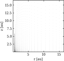
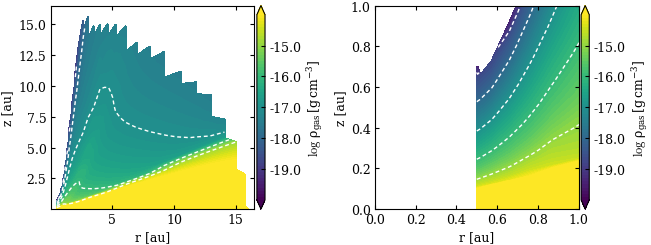
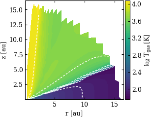
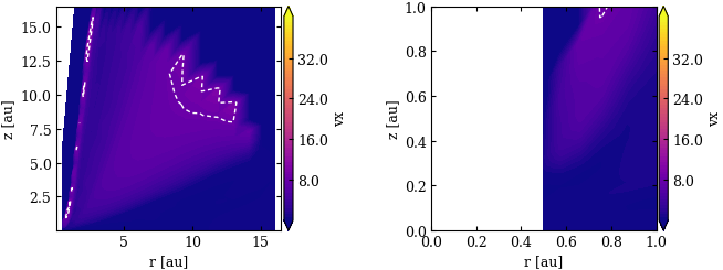
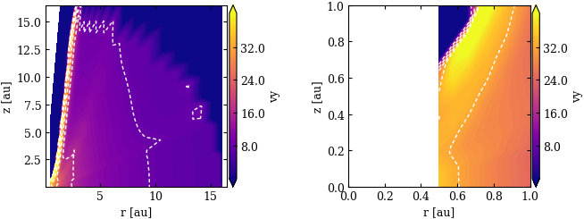
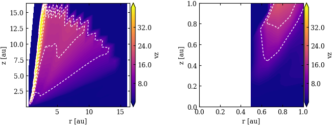
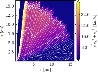
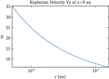
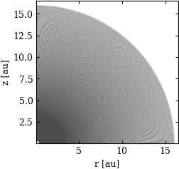
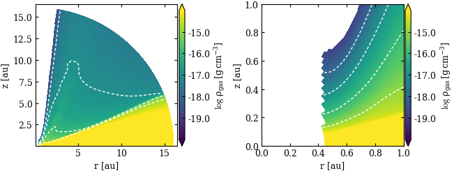
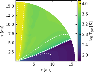
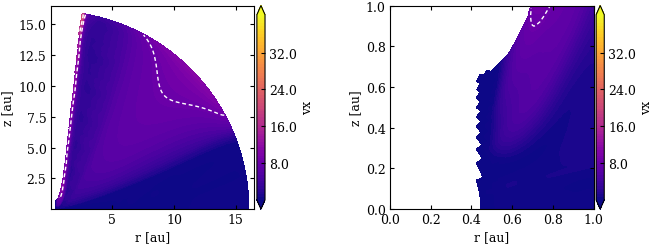
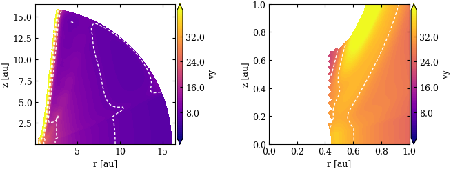
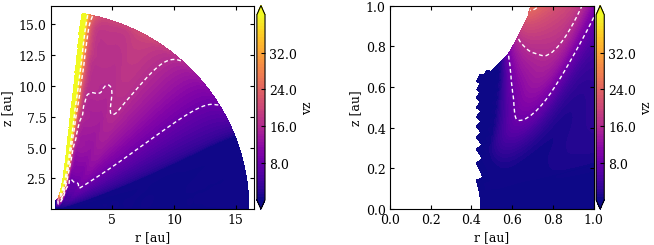
def plot_model(model):
"""
Plot various quantities of the MHD model using prodimopy plotting tools.
"""
pp = pplot.Plot(None)
xlim = [1.e-2, 16.5]
ylim = [1.e-2, 16.5]
constyle = {"zr": False, "xlog": False, "ylog": False, "axequal": True}
fig = pp.plot_grid(model, xlim=xlim, ylim=ylim, **constyle)
fig, axes = plt.subplots(1, 2, figsize=(6.7, 2.7))
pp.plot_cont(
model,
"rhog",
**constyle,
zlim=[1.0e-20, 1.0e-14],
extend="both",
ax=axes[0],
xlim=xlim,
ylim=ylim,
)
pp.plot_cont(
model,
"rhog",
**constyle,
zlim=[1.0e-20, 1.0e-14],
extend="both",
xlim=[0, 1],
ylim=[0, 1],
ax=axes[1],
)
fig.tight_layout()
fig = pp.plot_cont(model, "tg", **constyle, xlim=xlim, ylim=ylim)
for i, label in enumerate(["vx", "vy", "vz"]):
fig, axes = plt.subplots(1, 2, figsize=(7.0, 2.7))
pp.plot_cont(
model,
model.velocity[:, :, i],
label,
**constyle,
zlog=False,
extend="both",
zlim=[0, 40],
cmap="plasma",
ax=axes[0],
xlim=xlim,
ylim=ylim,
)
pp.plot_cont(
model,
model.velocity[:, :, i],
label,
**constyle,
zlog=False,
extend="both",
zlim=[0, 40],
xlim=[0, 1],
ylim=[0, 1],
cmap="plasma",
ax=axes[1],
)
fig.tight_layout()
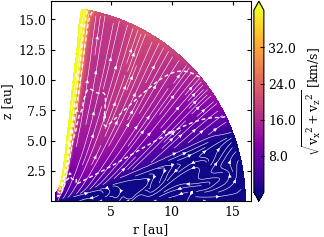
fig = pp.plot_cont(
model,
"velocity_xz",
**constyle,
zlog=False,
extend="both",
cmap="plasma",
zlim=[0, 40],
xlim=xlim,
ylim=ylim,
)
pp.streamplot_overlay(model, fig.axes[0], streamprops={"color": "white", "density": 1.5})
# Check the Keplerian velocity
fig = pp.plot_radial(
model,
model.velocity[:, :, 1],
"vy",
zidx=0,
ylog=False,
xlog=True,
ylim=[np.nanmin(model.velocity[:, 0, 1]), np.nanmax(model.velocity[:, 0, 1])],
title="Keplerian Velocity Vy at z=0 au",
)
plot_model(mhdpmodel)
PLOT: plot_grid ...
PLOT: plot_cont ...
PLOT: plot_cont ...
PLOT: plot_cont ...
PLOT: plot_cont ...
PLOT: plot_cont ...
PLOT: plot_cont ...
PLOT: plot_cont ...
PLOT: plot_cont ...
PLOT: plot_cont ...
PLOT: plot_cont ...
PLOT: plot_radial ...

Create the 2D input files for ProDiMo
[19]:
# Now do the conversion to ProDiMo, and create the pluto input files
# The MI2D_INIT model has a proper grid and parameters set up for ProDiMo. One needs to run it at least once with stop_after_init=.true.
# before using the toPorDiMo routine
pmodel = pread.read_prodimo("~/MODELS/prodimopy/MI2D_INIT",name="ProDiMo model")

# The toProDiMo routine does everything, however, it might be necessary to provide a special interpolation for your model.
# This then needs to be coded by yourself.
# The new 2D input files are written to the model directory (here MI2D_INIT)
newpmodel = mhd2DIn.toProDiMo(pmodel, outdir=pmodel.directory, fixmethod=3)
READ: StarSpectrum.out ...
READ: RTinterpolation.out ...
READ: Species.out ...
READ: ProDiMo.out: 100%|██████████| 2400/2400 [00:00<00:00, 19099.71it/s]
WARN: Could not open /home/rab/MODELS/prodimopy/MI2D_INIT/FlineEstimates.out!
READ: Elements.out ...
READ: dust_opac.out ...
READ: dust_sigmaa.out ...
READ: dust_opac_env.out ...
READ: dust_sigmaa.out ...
WARN: Could not open /home/rab/MODELS/prodimopy/MI2D_INIT/image.out!
READ: Parameter.out ...
INFO: Reading time:  0.28 s

Do the interpolation ...
- Interpolate rhoGas ...
- Interpolate velocity ...
- Interpolate tgas ...
Cutoff radius:  16.0
Found NaNs set them to zero.
Found NaNs set them to zero.
Found NaNs set them to zero.
Create the files ...
/home/rab/MODELS/prodimopy/MI2D_INIT/pluto_rho.dat
/home/rab/MODELS/prodimopy/MI2D_INIT/pluto_vx.dat
/home/rab/MODELS/prodimopy/MI2D_INIT/pluto_vy.dat
/home/rab/MODELS/prodimopy/MI2D_INIT/pluto_vz.dat
/home/rab/MODELS/prodimopy/MI2D_INIT/pluto_tgas.dat
Plot the interpolated ProDiMo model
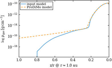
Even without running the ProDiMo model, one can directly use the new model (here newpmodel) to check if the interpolation worked as expected. Another way to have a quick look is to run the model now with interface2D=.true. and stop_after_init=.true. This way on can check if ProDiMo reads in the data correctly.
Please note the results here do not look very nice, as we use here a small number of grid points to speed things up. For a proper model nx,nz > 100 (or even more) is recommended.
[20]:
# Plot the new ProDiMo model
plot_model(newpmodel)
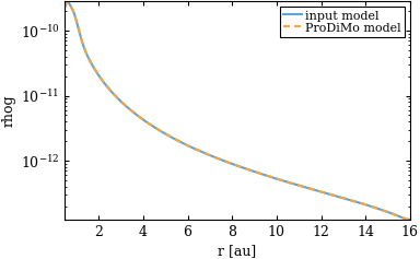
ppm = pplotm.PlotModels(styles=["-", "--"])
models = [mhdpmodel, newpmodel]
# We can directly compare the new intepolated numbers to the original MDH model
fig = ppm.plot_midplane(models, "rhog", "rhog")
# This plot shows some deviations, the reason is that we have to few vertical points, and most of them are concentrated towards the midplane
# where the interpolation is still accurate
fig = ppm.plot_vertical(models, 1, "rhog", "rhog", xlim=[1, 0])
PLOT: plot_grid ...
PLOT: plot_cont ...
PLOT: plot_cont ...
PLOT: plot_cont ...
PLOT: plot_cont ...
PLOT: plot_cont ...
PLOT: plot_cont ...
PLOT: plot_cont ...
PLOT: plot_cont ...
PLOT: plot_cont ...
PLOT: plot_cont ...
PLOT: plot_radial ...
PLOT: plot_midplane ...
PLOT: plot_vertical ...
0.0 11.43005 0.0 1.374635617264569e-10